Neural Architecture Search Part 5: Hardware-Aware NAS and Co-Design

We’ve traveled through NAS theory, search strategies, real-world applications, and efficient estimation techniques. But we’ve been operating under a hidden assumption: we optimize architectures for a generic “hardware” target.

In reality, neural networks don’t run on abstract computers—they run on specific devices: GPUs, CPUs, mobile phones, TPUs, and specialized edge accelerators. Each has unique characteristics that make certain architectures efficient and others inefficient. In this final part, we’ll explore how to design architectures aware of and optimized for specific hardware, and even co-design architecture and hardware together.

The Hardware Diversity Reality

Modern AI deployment spans an extraordinary range of devices:

A single “general-purpose” model is inherently inefficient:

• GPU Models: Optimize for parallelism and high throughput. Prefer operations that keep many cores busy.
• CPU Models: Optimize for sequential efficiency. Prefer operations with low memory bandwidth requirements and good cache utilization.
• Mobile Models: Optimize for power and memory. Prefer depthwise convolutions and reduced precision.
• Edge Accelerators: Designed for specific operations (e.g., INT8 quantization, particular layer types).

A general model might achieve 10% of peak hardware efficiency on each device, while specialized models achieve 70-80%.

Traditional NAS: Ignoring Hardware

Most NAS methods optimize for accuracy or generic MACs (multiply-accumulate operations). But remember from Part 4: MACs don’t directly predict real hardware performance.

The MACs Problem

Consider two architectures with identical MACs:

Architecture A: Large convolutions, high memory bandwidth requirements

• Theoretical (MACs): 1 billion operations
• Actual GPU latency: 100ms (CPU bottleneck, memory bandwidth limited)
• GPU efficiency: 45%

Architecture B: Depthwise separable convolutions, low memory bandwidth

• Theoretical (MACs): 1 billion operations
• Actual GPU latency: 30ms (better memory access patterns)
• GPU efficiency: 85%

Same MACs, but 3× different latency! Standard NAS would treat them as equivalent.

Hardware-Aware NAS: The Solution

Hardware-aware NAS includes actual hardware latency measurements in the search objective.

The Approach

Rather than optimizing purely for accuracy:

\[\text{maximize} \quad \text{Accuracy}\]

We optimize for accuracy subject to hardware constraints:

\(\text{maximize} \quad \text{Accuracy}\) \(\text{subject to} \quad \text{Latency}_{\text{target device}} \leq \text{Budget}\)

Practical Implementation

1. Profile Operations: Measure latency of each primitive operation on target hardware
   • What’s the actual latency of a $3 \times 3$ convolution?
   • What’s the latency of depthwise convolution?
   • How do different quantization schemes affect latency?
2. Build Latency Predictor: Train a model that predicts architecture latency from its structure
   • Input: Architecture description
   • Output: Predicted latency on target device
   • Learns from profiling measurements
3. Include in Search Objective: Use latency predictions to guide architecture search
   • Prioritize architectures that meet latency budgets
   • Avoid wasting search time on architectures that violate constraints
   • Focus search on the accuracy-latency Pareto frontier

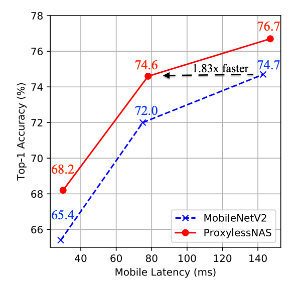
Results: Architecture Specialization

Hardware-aware NAS discovers radically different architectures for different targets:

For GPU (high parallelism):

• Larger kernels (5×5, 7×7)
• More channels per layer
• Deep networks with wide layers

For CPU (sequential efficiency):

• Smaller kernels (1×1, 3×3)
• Depthwise/grouped convolutions
• Shallower networks with good cache behavior

For Mobile (power and memory):

• Depthwise separable convolutions
• Channel reductions via 1×1
• Skip connections to reduce retraining
• Quantization-friendly operations

The same search algorithm discovers different architectures when constrained by different hardware targets. This is the power of hardware-aware NAS.

Many-Objective NAS: Beyond Accuracy-Latency

While accuracy-latency trade-off is powerful, real systems often have multiple competing objectives:

Objectives:

• Accuracy: Maximize validation accuracy
• Latency: Minimize inference time
• Memory: Minimize model size and activation memory
• Energy: Minimize power consumption
• Fairness: Ensure model doesn’t discriminate
• Robustness: Maintain accuracy under adversarial inputs

The Pareto Frontier

Rather than finding a single “best” architecture, many-objective NAS finds the Pareto frontier—the set of architectures where improving one objective requires sacrificing another.

For example, among models meeting a latency constraint:

• Architecture A: 85% accuracy, 100MB memory
• Architecture B: 82% accuracy, 40MB memory
• Architecture C: 84% accuracy, 60MB memory

All are on the Pareto frontier. The choice depends on additional constraints (available memory, required accuracy).

Modern NAS systems return sets of architectures at different efficiency-accuracy trade-offs, letting deployment engineers choose based on specific constraints.

Neural-Hardware Architecture Co-Design

The ultimate frontier: instead of designing architecture for fixed hardware or hardware for fixed architecture, co-design both together.

Traditional Separate Optimization

Step 1: Designers propose hardware specification
        ↓
Step 2: NAS finds optimal architecture for that hardware
        ↓
(Problem: Hardware may not be optimal for discovered architecture)

Co-Design: Joint Optimization

Step 1: Define design space for both architecture and hardware
Step 2: Jointly search over (architecture, hardware) pairs
Step 3: Evaluate each pair's performance
Step 4: Find Pareto-optimal configurations
        ↓
(Result: Architectures and hardware designed for each other)

Co-Design Benefits

Joint optimization discovers synergies:

• Certain architectures enable more efficient hardware implementation
• Custom hardware can efficiently implement specific operations
• Architecture-hardware pairs achieve higher efficiency than separate optimizations

Example:

• Neural network heavily uses depthwise convolution
• Co-design might discover that adding a specialized depthwise unit to hardware accelerates that operation significantly
• This specialized unit is cheap to add and benefits many architectures
• Result: 20% efficiency gain that separate optimization would miss

Practical Co-Design Dimensions

Architecture variables:

• Operation types and configurations
• Layer depths and widths
• Skip connection patterns
• Quantization schemes

Hardware variables:

• Memory hierarchy (cache sizes, bandwidth)
• Compute units (ALUs, multipliers)
• Specialized functional units
• Data movement optimizations
• Parallelism structure

From General to Specialized: The Transformation

Hardware-aware and co-design NAS enable a fundamental shift:

Case Study: Mobile Deployment

Traditional approach:

• Train one large model (ResNet-50, 100MB)
• Compress it (quantization, pruning, distillation)
• Deploy everywhere
• Poor efficiency on each device (30-50% of peak)

Hardware-aware NAS approach:

• Run NAS targeting mobile CPU latency budget (< 50ms)
• Discover MobileNetV3 architecture
• Result: 5MB model, 50ms latency, 75% accuracy
• Efficiency: 75% of peak mobile performance
• Size: 20× smaller than compressed ResNet

Beyond Vision: NAS for Other Domains

Hardware-aware NAS is proving valuable across machine learning:

NLP and Language Models

Hardware-aware NAS for transformers discovers:

• Optimal attention head dimensions for specific accelerators
• Efficient token sequence handling
• Quantization schemes for transformer operations
• Sparse attention patterns that match hardware capabilities

Result: 2-3× speedup in language model inference compared to general BERT/GPT.

Generative Models (GANs)

NAS has been applied to GAN architecture search, discovering:

• Generator architectures with minimal parameters while maintaining quality
• Discriminator designs optimized for convergence speed
• Hardware-efficient operations that produce high-quality images

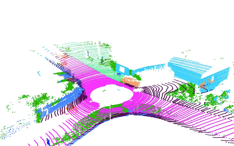
Point Cloud and 3D

For 3D perception (autonomous vehicles, AR):

• Search for efficient point cloud networks
• Optimize for specific 3D accelerators
• Balance between spatial locality and semantic understanding

Zero-Cost NAS: The Latest Frontier

We discussed zero-shot NAS briefly in Part 3, but it deserves deeper exploration. Zero-cost proxies enable NAS without training super-networks at all.

The insight: we can estimate architecture quality without any training by measuring properties like:

• Gradient flow (synaptic saliency)
• Spectral properties of initialization
• Activation diversity
• Fisher information

These proxies compute in milliseconds and remarkably well predict which architectures will be accurate.

Impact of Zero-Cost NAS

Computational cost: From 22,400 GPU-hours (original NAS) to 1-2 GPU hours for zero-cost approaches

Who can run NAS?

• Original: Major companies with supercomputers
• Today: Any research lab with a single GPU
• Tomorrow: Researchers on laptops using zero-cost methods

This democratization is transforming NAS from a research curiosity to a practical tool.

Practical Hardware-Aware NAS Workflow

Here’s how practitioners actually run hardware-aware NAS today:

1. Define constraints (latency, memory, power budget for target device)

2. Profile operations on target hardware
   • Measure $1 \times 1$, $3 \times 3$, $5 \times 5$ convolutions
   • Measure pooling, activation functions, batch norm
   • Account for kernel implementation and overhead
3. Train latency predictor
   • Sample random architectures
   • Measure their latency on device
   • Train model: architecture → latency
4. Run NAS with latency constraints
   • Use weight-sharing super-network (Part 4)
   • Include latency prediction in search objective
   • Search until convergence
5. Validate and deploy
   • Fine-tune top candidates
   • Profile on actual target device
   • Deploy with real measurements

The Impact

Hardware-aware NAS has transformed what’s possible:

• Google Pixel: Uses EfficientNet optimized for Snapdragon processor
• Apple Neural Engine: Models architected for specific mobile accelerators
• Tesla: Computer vision models tuned for specific hardware in vehicles
• Edge devices: Custom models for smart speakers, security cameras, IoT

Conclusion: From Generic to Specialized

Over five parts, we’ve traced NAS from theoretical concept to practical tool:

1. Part 1: Understood the foundations (operations, building blocks, efficiency-accuracy trade-off)
2. Part 2: Learned how to search (search spaces, strategies)
3. Part 3: Saw real-world impact (EfficientNet, MobileNets, beyond vision)
4. Part 4: Discovered efficiency tricks (weight sharing, ProxylessNAS)
5. Part 5: Embraced hardware reality (hardware-aware NAS, co-design, democratization)

The key evolution: from “one architecture for all hardware” to “specialized architectures for specific hardware and constraints.”

This specialization unlocks dramatic efficiency gains:

• 10-100× smaller models
• 10-50× faster inference
• 5-20× lower power consumption
• Better accuracy within constraints

Hardware-aware NAS represents the future of deep learning deployment: AI systems designed holistically from task, to architecture, to hardware—each optimized for the others.

---

Series Navigation:

• Part 1: Foundations and Building Blocks
• Part 2: Search Spaces and Strategies
• Part 3: Applications and Real-World Impact
• Part 4: Efficient Estimation Strategies
• Part 5: Hardware-Aware NAS and Co-Design (this post)

---

References:

• MIT 6.5940: TinyML and Efficient Deep Learning - Lecture 8: Neural Architecture Search Part II (Fall 2024)
• HAQ: Hardware-Aware Automated Quantization (Wang et al., CVPR 2019) - Hardware-aware optimization
• FairDARTS: Eliminating Unfair Advantages in Differentiable Architecture Search (Chu et al., ECCV 2020) - Fair comparison across hardware
• Exploring the Limits of Transfer Learning with a Unified Text-to-Text Transformer (Raffel et al., JMLR 2020) - Multi-objective optimization
• Zero-Cost Proxies for Lightweight NAS (Abdelfattah et al., ICLR 2021) - Zero-cost NAS
• NAS-Evaluation-is-Frustratingly-Hard - Challenges in evaluating NAS
• AutoML: A Survey of the State-of-the-Art (Hutter et al., KDD 2019) - Comprehensive AutoML overview including NAS