Neural Architecture Search Part 1: Foundations and Building Blocks
Neural Architecture Search (NAS) is one of the most exciting developments in deep learning—a technique that automates the design of neural network architectures rather than relying on human engineers to manually craft them. In this first part, we’ll explore the foundations, understand why NAS matters, and learn about the building blocks that form the basis of modern neural networks.
The Challenge of Manual Architecture Design
Designing neural network architectures is hard. For decades, engineers spent countless hours experimenting with different layer configurations, testing various depths, widths, and connection patterns. ResNet, MobileNet, EfficientNet—these breakthrough architectures were often discovered through manual exploration and intuition.
But here’s the problem: what works for image classification might not work for speech recognition. What’s efficient on a GPU might be terrible on a mobile phone. The search space is enormous, and manual design doesn’t scale.
This is where Neural Architecture Search comes in. Instead of humans designing architectures by hand, we can use automated algorithms to explore the design space and discover architectures optimized for specific constraints and datasets.
Understanding the Efficiency-Accuracy Trade-off
Before diving into NAS, we need to understand a fundamental tension in deep learning: the trade-off between model efficiency and accuracy.

Every neural network must balance three critical dimensions:
Storage: How much memory does the model occupy? Smaller models fit on devices with limited memory (phones, embedded systems).
Latency: How fast can the model make predictions? Faster inference means better user experience and lower computational costs.
Energy: How much power does the model consume? This matters for battery-powered devices and data center efficiency.
The catch: larger models with more layers and parameters typically achieve higher accuracy, but they consume more storage, latency, and energy. Smaller, efficient models are fast and use less energy but may sacrifice accuracy.
NAS helps us find the sweet spot—architectures that achieve excellent accuracy while meeting specific efficiency constraints.
Recap: Primitive Operations
Before we talk about search strategies, we need to understand the building blocks that form all neural networks. These primitive operations are like the alphabet of deep learning.
Fully Connected Layer (Linear Layer)
A fully connected layer is the simplest neural network operation. Every input is connected to every output through a weight matrix.
For a layer with $c_i$ input channels, $c_o$ output channels, and batch size $n$:
\[\text{MACs} = c_o \cdot c_i\](We measure complexity in Multiply-Accumulate operations, or MACs, for a batch size of 1)
Convolution Layer
Convolution is the foundation of modern deep learning, especially for image tasks. Instead of connecting every input to every output, convolution uses small kernels that slide across the input.
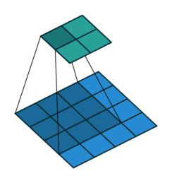
For a convolution with:
- Input channels: $c_i$
- Output channels: $c_o$
- Kernel height/width: $k_h, k_w$
- Input/output height/width: $h_i, h_o, w_i, w_o$
The computational cost is:
\[\text{MACs} = c_o \cdot c_i \cdot k_h \cdot k_w \cdot h_o \cdot w_o\]This is significantly more efficient than a fully connected layer for spatial data like images.
Grouped Convolution
Grouped convolution splits the input channels into groups and applies separate convolutions to each group. This reduces computation compared to standard convolution.
For $g$ groups:
\[\text{MACs} = \frac{c_o \cdot c_i \cdot k_h \cdot k_w \cdot h_o \cdot w_o}{g}\]Depthwise Convolution
Depthwise convolution is an extreme case of grouped convolution where each input channel gets its own kernel ($g = c_i = c_o$).
\[\text{MACs} = c_o \cdot k_h \cdot k_w \cdot h_o \cdot w_o\]This is extremely efficient because the computation scales with kernel size and spatial dimensions, not with channel dimensions.
1x1 Convolution
A special case of convolution using $1 \times 1$ kernels. These operations are pure channel transformations without spatial processing.
\[\text{MACs} = c_o \cdot c_i \cdot h_o \cdot w_o\]Classic Building Blocks: ResNet Bottleneck
While primitive operations are the atoms, modern architectures combine them into reusable blocks. The ResNet bottleneck block is a perfect example.
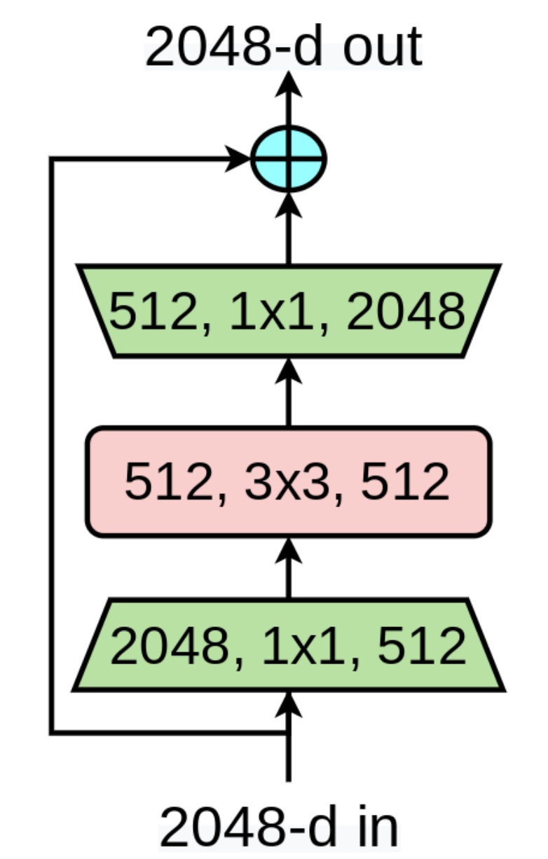
The bottleneck block works in three steps:
- Reduce Channels: Use a $1 \times 1$ convolution to reduce the number of channels by 4× (e.g., from 2048 to 512)
- Spatial Processing: Apply a standard $3 \times 3$ convolution on the reduced feature map
- Expand Channels: Use another $1 \times 1$ convolution to expand back to the original channel count
This design is clever: the bottleneck reduces computation in the expensive $3 \times 3$ convolution while maintaining representational capacity through the channel expansions.
Why Building Blocks Matter
Instead of treating each layer as an independent choice, NAS searches over combinations of blocks like the bottleneck. This dramatically reduces the search space because:
- We don’t need to choose layer-by-layer
- We leverage human-discovered building blocks that we know work well
- The search can focus on higher-level decisions: how many blocks, what dimensions, what connections
Looking Ahead
We now understand the foundations: the efficiency challenges that motivate NAS, the primitive operations that form all networks, and the building blocks that modern architectures use. In Part 2, we’ll dive into the core of NAS: how to design the search space and what strategies we can use to explore it effectively.
Series Navigation:
- Part 1: Foundations and Building Blocks (this post)
- Part 2: Search Spaces and Strategies
- Part 3: Applications and Real-World Impact
- Part 4: Efficient Estimation Strategies
- Part 5: Hardware-Aware NAS and Co-Design
References:
- MIT 6.5940: TinyML and Efficient Deep Learning - Lecture 7: Neural Architecture Search Part I (Fall 2024)
- Deep Residual Learning for Image Recognition (He et al., CVPR 2016) - Introduces ResNet and bottleneck blocks
- MobileNets: Efficient Convolutional Neural Networks for Mobile Vision Applications (Howard et al., 2017)