Quantization Part 8: Mixed-Precision Quantization

Throughout this series, we’ve explored uniform quantization strategies—applying the same bit-width (8-bit, 4-bit, or even 1-bit) to all layers. But neural networks are not uniform. Some layers are highly sensitive to quantization, while others tolerate extreme compression. The first convolutional layer processes raw pixel data and needs fine-grained precision; batch normalization layers are robust and work well at 4 bits; the final classifier layer determines class boundaries and benefits from higher precision. This heterogeneity motivates mixed-precision quantization: assigning different bit-widths to different layers based on their individual sensitivity and computational cost.

The challenge? With dozens of layers and multiple precision choices per layer, the search space explodes combinatorially. Manual exploration is infeasible. This is where Hardware-Aware Automated Quantization (HAQ) enters: a reinforcement learning approach that automatically discovers optimal per-layer bit-width configurations while respecting hardware constraints like model size, latency, and energy consumption.

The Mixed-Precision Design Space

Why Uniform Quantization Is Suboptimal

Consider a typical ResNet-50:

Layer sensitivity analysis:

Layer Type	Quantization Sensitivity	Reason
First Conv	High	Processes raw pixels with subtle patterns
Early Residual Blocks	High	Low-level features (edges, textures) need precision
Middle Residual Blocks	Medium	Mid-level features more robust to quantization
Late Residual Blocks	Low	High-level semantic features tolerate compression
Batch Normalization	Very Low	Normalization statistics inherently robust
Final Classifier	High	Small changes in logits dramatically affect predictions

Uniform INT8: Wastes bits on robust layers, underserves sensitive layers.

Optimal strategy: Allocate more bits to sensitive layers, fewer to robust layers.

The Combinatorial Explosion

For a 50-layer network with 4 precision choices {2, 4, 6, 8 bits}:

\[\text{Total configurations} = 4^{50} \approx 10^{30}\]

Exhaustive search is impossible. Even evaluating one configuration (training + validation) takes hours. We need a smart search strategy.

HAQ: Hardware-Aware Automated Quantization

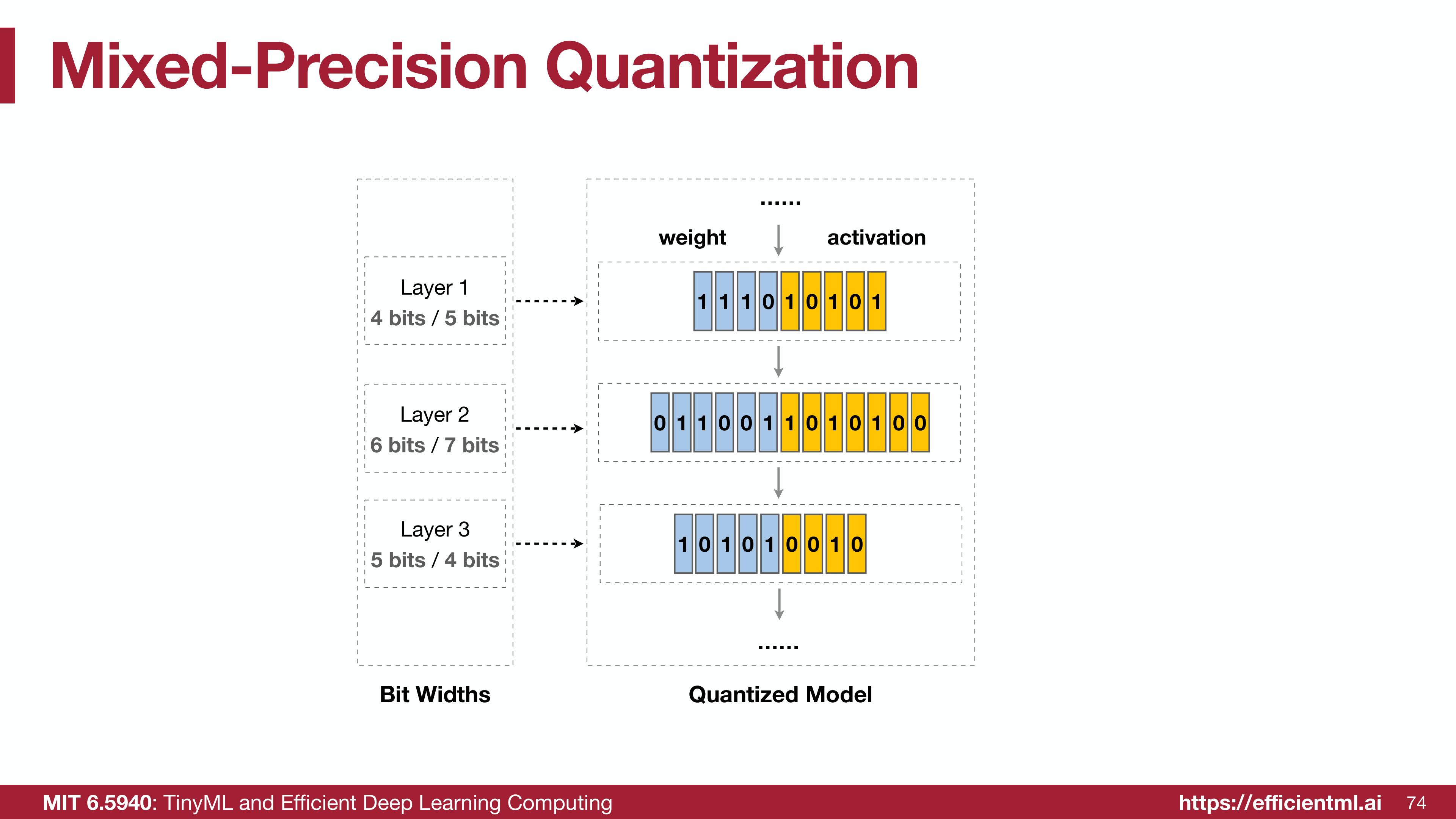HAQ uses reinforcement learning to search for optimal mixed-precision policies

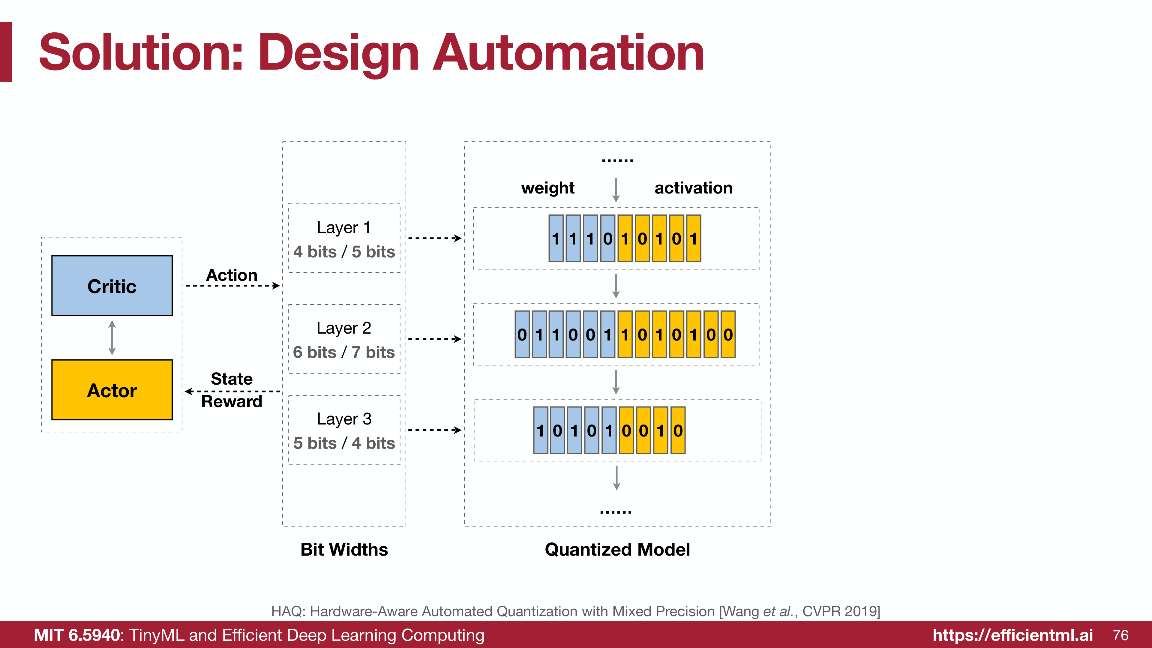
HAQ framework (Wang et al., 2019) formulates mixed-precision search as a reinforcement learning (RL) problem:

Agent: RL policy network that outputs bit-width decisions

State: Layer characteristics (depth, channels, kernel size, sensitivity)

Action: Bit-width choice for current layer {2, 4, 6, 8}

Reward: Accuracy improvement relative to hardware cost (latency, size, energy)

Goal: Find policy that maximizes accuracy subject to resource constraints

The RL Formulation

State representation $s_t$ for layer $t$:

\[s_t = [d_t, c_{\text{in}}, c_{\text{out}}, k, \text{stride}, \text{sensitivity}_t, \text{current\_size}, \text{current\_latency}]\]

where:

• $d_t$: Layer depth (position in network)
• $c_{\text{in}}, c_{\text{out}}$: Input/output channels
• $k$: Kernel size
• $\text{sensitivity}_t$: Empirically measured quantization sensitivity
• $\text{current_size}$: Cumulative model size so far
• $\text{current_latency}$: Cumulative inference latency

Action $a_t$: Bit-width choice $\in {2, 4, 6, 8}$ for layer $t$

Policy $\pi_\theta(a_t

s_t)$: Neural network that outputs probability distribution over bit-widths given state

Trajectory: Sequence of decisions for all layers:

\[\tau = [(s_1, a_1), (s_2, a_2), \ldots, (s_L, a_L)]\]

where $L$ is total number of layers.

Reward function:

\[R(\tau) = \begin{cases} \text{Accuracy}(\tau) & \text{if } \text{Constraint}(\tau) \leq \text{Budget} \\ -\infty & \text{otherwise} \end{cases}\]

Constraint can be:

• Model size: $\sum_{t=1}^{L} \text{size}t(a_t) \leq \text{Budget}{\text{size}}$
• Latency: $\sum_{t=1}^{L} \text{latency}t(a_t) \leq \text{Budget}{\text{latency}}$
• Energy: $\sum_{t=1}^{L} \text{energy}t(a_t) \leq \text{Budget}{\text{energy}}$

Objective: Learn policy $\pi_\theta$ that maximizes expected reward:

\[\theta^* = \arg\max_\theta \mathbb{E}_{\tau \sim \pi_\theta} [R(\tau)]\]

Training the RL Agent

1. Sample trajectories from current policy $\pi_\theta$:

for episode in range(num_episodes):
    state = initial_state()
    trajectory = []
    
    for layer in network.layers:
        # Agent chooses bit-width
        action = policy_network.sample(state)
        
        # Update state with action's resource cost
        next_state = update_state(state, action)
        trajectory.append((state, action))
        state = next_state
    
    # Evaluate configuration
    accuracy = train_and_evaluate(trajectory)
    constraint_satisfied = check_constraints(trajectory)
    reward = accuracy if constraint_satisfied else -inf
    
    # Store trajectory and reward
    memory.append((trajectory, reward))

2. Update policy using REINFORCE algorithm:

\[\nabla_\theta J(\theta) = \mathbb{E}_{\tau \sim \pi_\theta} \left[ \sum_{t=1}^{L} \nabla_\theta \log \pi_\theta(a_t | s_t) \cdot R(\tau) \right]\]

With baseline $b$ (average reward) to reduce variance:

\[\nabla_\theta J(\theta) = \mathbb{E}_{\tau \sim \pi_\theta} \left[ \sum_{t=1}^{L} \nabla_\theta \log \pi_\theta(a_t | s_t) \cdot (R(\tau) - b) \right]\]

3. Repeat until convergence or budget exhausted.

Sensitivity-Aware State Representation

A critical component is layer sensitivity, which guides the RL agent toward good decisions.

Measuring sensitivity:

1. Start with FP32 baseline accuracy $A_{\text{FP32}}$
2. For each layer $i$, quantize only that layer to target bit-width $b$
3. Measure accuracy drop: $\Delta A_i(b) = A_{\text{FP32}} - A_i(b)$
4. Sensitivity: $S_i(b) = \Delta A_i(b)$

High sensitivity ($S_i$ large): Layer needs higher precision

Low sensitivity ($S_i$ small): Layer tolerates lower precision

This sensitivity is included in the state $s_t$, helping the agent make informed decisions without random exploration.

Per-layer sensitivity guides bit-width assignment

Hardware Cost Models

HAQ requires accurate models of how bit-width choices affect hardware metrics.

Model Size

For layer $t$ with:

• $c_{\text{in}}$ input channels
• $c_{\text{out}}$ output channels
• Kernel size $k \times k$
• Bit-width $b_t$

Parameter count:

\[P_t = c_{\text{out}} \cdot c_{\text{in}} \cdot k^2\]

Memory (bytes):

\[M_t(b_t) = P_t \cdot \frac{b_t}{8}\]

Total model size:

\[M_{\text{total}} = \sum_{t=1}^{L} M_t(b_t)\]

Latency

Latency depends on:

• Data movement: Memory access time (proportional to bit-width)
• Computation: MAC operations (bit-width affects efficiency)

Simplified latency model:

\[T_t(b_t) = \alpha \cdot \frac{b_t}{8} \cdot P_t + \beta \cdot \text{MAC}_t \cdot f(b_t)\]

where:

• $\alpha$: Memory bandwidth coefficient
• $\beta$: Compute throughput coefficient
• $f(b_t)$: Bit-width-dependent MAC efficiency

For INT8, $f(8) = 1$; for INT4, $f(4) \approx 0.3$ (hardware-dependent).

Energy

Energy combines memory access and computation:

\[E_t(b_t) = E_{\text{mem}}(b_t) + E_{\text{comp}}(b_t)\]

Memory energy:

\[E_{\text{mem}}(b_t) = \frac{b_t}{8} \cdot P_t \cdot e_{\text{mem}}\]

where $e_{\text{mem}}$ is energy per byte (e.g., 640 pJ/byte for DRAM).

Compute energy:

\[E_{\text{comp}}(b_t) = \text{MAC}_t \cdot e_{\text{MAC}}(b_t)\]

where $e_{\text{MAC}}(b_t)$ is bit-width-dependent MAC energy:

Bit-width	Energy per MAC
FP32	4.6 pJ
INT16	1.1 pJ
INT8	0.2 pJ
INT4	0.05 pJ
INT2	0.01 pJ

These hardware cost models are platform-specific and must be calibrated for target deployment hardware (GPU, CPU, FPGA, edge TPU).

HAQ Training Pipeline

Complete HAQ pipeline: RL search + QAT fine-tuning

Phase 1: RL-Based Search

Objective: Quickly explore configurations, identify promising candidates.

Details:

• Policy network: 2-layer LSTM with 300 hidden units
• Training: 1000-2000 episodes
• Each episode: Sample one configuration, evaluate accuracy (simplified)
• Accuracy evaluation: Short QAT fine-tuning (5-10 epochs)
• Time: 1-2 days on GPU cluster

Output: Top-K configurations (e.g., K=10) that satisfy constraints.

Phase 2: Full QAT Fine-Tuning

Objective: Fully train the best configurations from Phase 1.

Details:

• Select best configuration from RL search
• QAT fine-tuning: 50-100 epochs with full training pipeline
• Learning rate schedule: cosine annealing
• Data augmentation: full training recipe
• Time: 2-3 days per configuration

Output: Final quantized model ready for deployment.

Constraint Handling

Hard constraints: If constraint violated, set reward = $-\infty$ (configuration rejected).

Soft constraints: Use Lagrangian relaxation to balance accuracy and resource cost:

\[R(\tau) = \text{Accuracy}(\tau) - \lambda \cdot \max(0, \text{Cost}(\tau) - \text{Budget})\]

where $\lambda$ is a penalty coefficient.

Dynamic $\lambda$ adjustment: If too many configurations violate constraints, increase $\lambda$; if too few, decrease $\lambda$.

HAQ Results on ImageNet

ResNet-50 Compression

Baseline: FP32 ResNet-50

• Accuracy: 76.1% Top-1
• Model size: 97.5 MB
• Latency: 35 ms (GPU), 120 ms (CPU)

HAQ-optimized configurations:

Target	Accuracy	Model Size	Latency (CPU)	Speedup
0.5× latency	75.3% (−0.8%)	52 MB	60 ms	2.0×
0.3× latency	73.7% (−2.4%)	28 MB	36 ms	3.3×
0.2× latency	71.2% (−4.9%)	18 MB	24 ms	5.0×

Comparison with uniform quantization:

Method	Target Size	Accuracy	Latency
Uniform INT8	24.4 MB	75.8%	42 ms
Uniform INT6	18.3 MB	72.1%	35 ms
HAQ (mixed)	18.0 MB	73.7%	28 ms

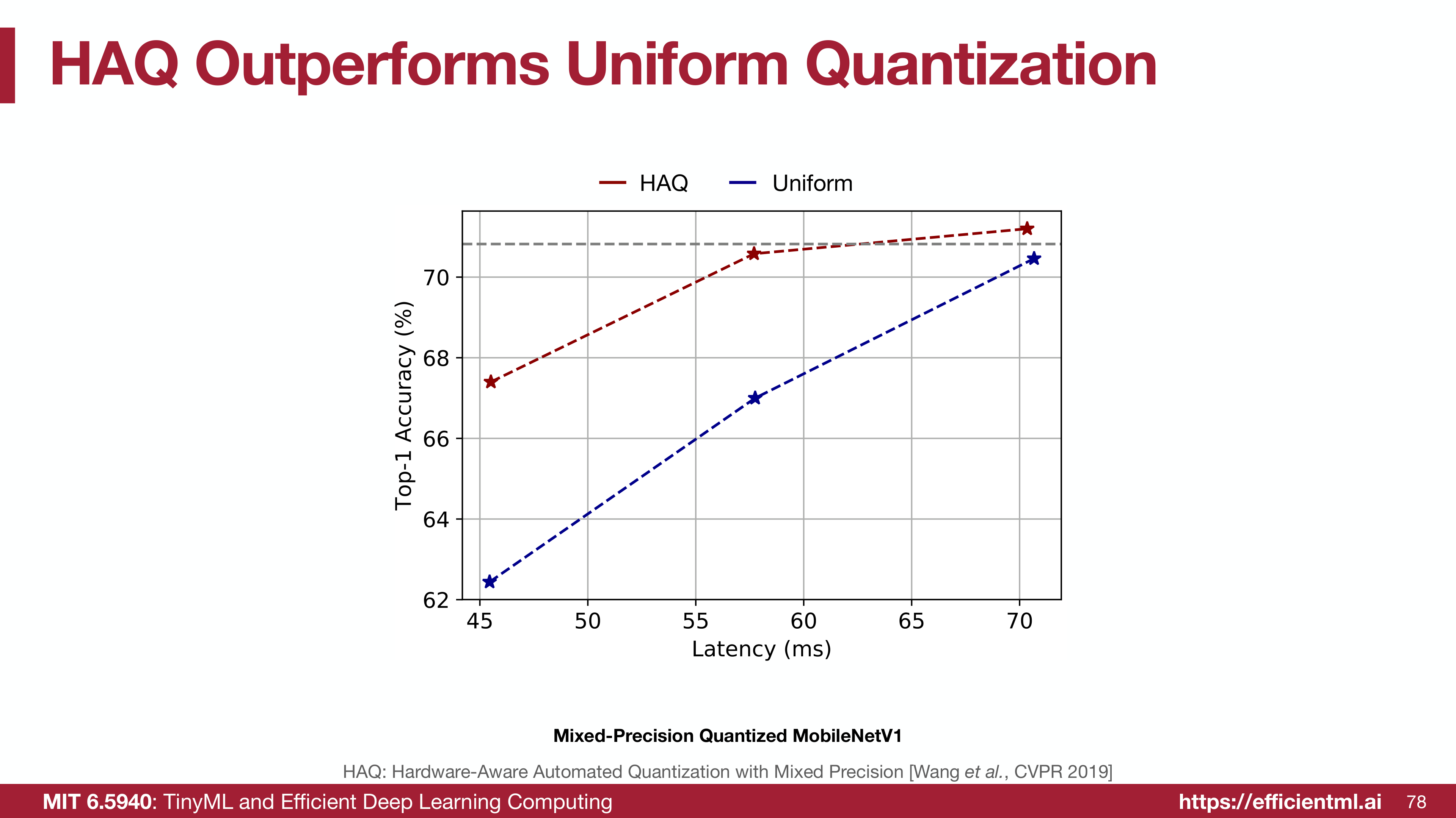
Observation: HAQ achieves 1.6% higher accuracy than uniform INT6 at similar model size, and 20% lower latency.

MobileNetV2 Optimization

Baseline: FP32 MobileNetV2

• Accuracy: 71.9% Top-1
• Model size: 14 MB
• Latency: 15 ms (GPU)

HAQ results:

Constraint	Accuracy	Size	Bit-width Distribution
4 MB budget	70.1%	3.8 MB	{2, 4, 6, 8} heavily skewed to 2-4 bits
6 MB budget	71.2%	5.9 MB	{4, 6, 8} majority 4-6 bits
8 MB budget	71.6%	7.8 MB	{4, 6, 8} majority 6-8 bits

Key finding: HAQ automatically discovers that:

• First layer: 8 bits (high sensitivity)
• Depthwise convolutions: 2-4 bits (robust)
• Pointwise convolutions: 4-6 bits (moderate sensitivity)
• Final classifier: 8 bits (high sensitivity)

This layer-wise pattern emerges from RL training without manual specification!

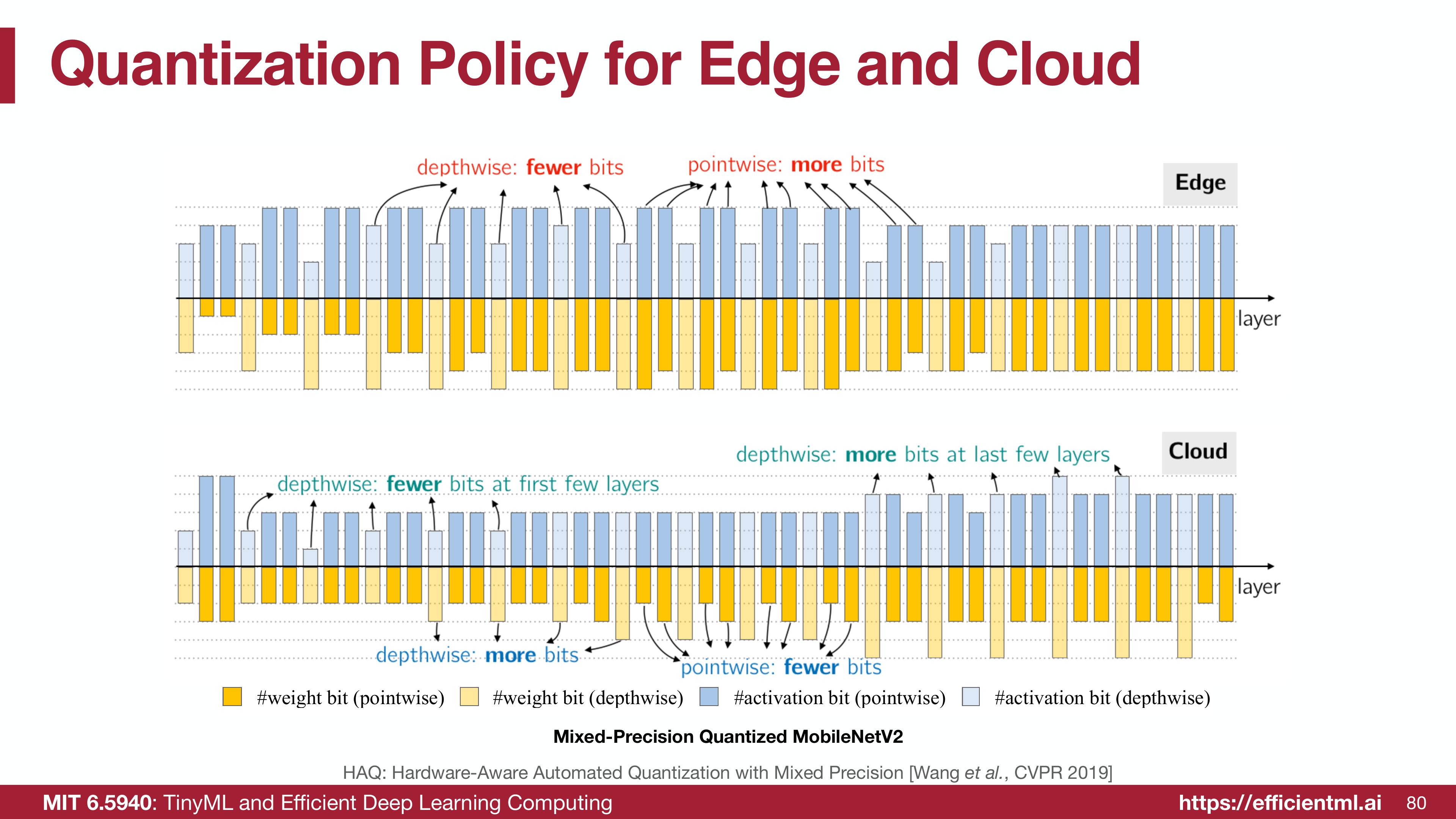HAQ-discovered bit-width assignments show clear patterns: first/last layers get higher precision

Learned Bit-Width Patterns

Across multiple networks, HAQ consistently discovers similar patterns:

Pattern 1: First Layer High Precision

Why: Processes raw input (pixels, audio waveforms) with subtle patterns that require fine-grained discrimination.

Typical assignment: 8 bits

Pattern 2: Early Layers Higher Precision

Why: Low-level features (edges, textures, frequency components) are building blocks for higher layers. Errors here propagate through the network.

Typical assignment: 6-8 bits

Pattern 3: Middle Layers Lower Precision

Why: Mid-level features are more abstract and robust to quantization noise.

Typical assignment: 4-6 bits

Pattern 4: Final Layers High Precision

Why: Classification logits or regression outputs are directly used for decisions. Small errors can cause incorrect predictions.

Typical assignment: 8 bits

Pattern 5: Batch Normalization Layers Minimal Precision

Why: BN parameters (mean, variance, scale, shift) are applied to normalized distributions. Quantization has minimal impact.

Typical assignment: 2-4 bits (sometimes even 1 bit!)

Pattern 6: Depthwise Separable Convolutions Lower Precision

Why: Depthwise convolutions have fewer parameters and are inherently more robust.

Typical assignment: 2-4 bits

Advanced HAQ Extensions

Multi-Objective Optimization

Optimize multiple hardware metrics simultaneously:

\[R(\tau) = w_1 \cdot \text{Accuracy} - w_2 \cdot \frac{\text{Latency}}{\text{Budget}_{\text{latency}}} - w_3 \cdot \frac{\text{Energy}}{\text{Budget}_{\text{energy}}}\]

Pareto frontier: HAQ can generate multiple configurations representing different accuracy-efficiency trade-offs.

Channel-Level Mixed Precision

Extend to per-channel bit-widths within a layer:

State: Include per-channel sensitivity

Action: Assign bit-widths to channel groups

Challenge: Combinatorial explosion worsens. Use hierarchical RL or group channels.

Hardware-in-the-Loop

Measure actual hardware performance rather than using analytical models:

def evaluate_latency(config):
    # Deploy config to target hardware
    model = build_quantized_model(config)
    model.deploy_to_hardware(target_device)
    
    # Measure real latency
    latency = model.benchmark(input_data, iterations=1000)
    return latency

Benefit: Accounts for hardware-specific optimizations (caching, pipelining, parallelism).

Cost: Much slower evaluation (hours per configuration).

Transfer Learning Across Networks

Train RL agent on one network (e.g., ResNet-50), transfer to similar architectures (ResNet-101, ResNet-152):

State representation: Use normalized layer characteristics (relative depth, channel ratios)

Transfer: Pretrain policy on smaller network, fine-tune on larger network

Speedup: Reduces search time by 50-70%.

Comparison with Other AutoML Methods

Neural Architecture Search (NAS)

Difference: NAS searches for network architecture (layer types, connections); HAQ searches for bit-widths given fixed architecture.

Complementary: Can combine NAS + HAQ for joint architecture and quantization search.

Bayesian Optimization

Approach: Model accuracy as Gaussian process, use acquisition function to select next configuration.

Comparison:

• BO: Sample-efficient but struggles with high-dimensional spaces
• HAQ (RL): Handles combinatorial spaces better, leverages layer structure

Evolutionary Algorithms

Approach: Mutation and crossover of bit-width configurations, survival of the fittest.

Comparison:

• EA: Simple, parallelizable
• HAQ (RL): More sample-efficient due to learned policy

Manual Search with Heuristics

Approach: Manually analyze layer sensitivity, assign bit-widths based on rules.

Comparison:

• Manual: Fast but suboptimal, requires expert knowledge
• HAQ: Automated, discovers patterns humans might miss

Practical Deployment Considerations

Hardware Support

Not all hardware supports arbitrary mixed-precision:

GPUs: Typically support {FP32, FP16, INT8}, limited INT4

CPUs: {FP32, INT8}, INT4 via specialized libraries

Edge TPUs: {INT8, INT16}, fixed-function accelerators

FPGAs: Fully flexible bit-widths, but require custom design

Recommendation: Constrain HAQ search to hardware-supported bit-widths.

Software Frameworks

TensorFlow Lite: Supports per-channel INT8, limited mixed-precision

PyTorch Mobile: Supports INT8, experimental INT4

ONNX Runtime: Supports INT8, limited mixed-precision

TVM: Flexible AutoTVM for mixed-precision compilation

Recommendation: Verify target framework supports discovered configuration before deployment.

Quantization Granularity

Layer-level: Easiest to implement, good balance

Channel-level: Higher accuracy, more complex implementation

Weight-level: Maximum flexibility, impractical for most hardware

Recommendation: Start with layer-level, extend to channel-level for critical accuracy gains.

Limitations and Future Directions

Current Limitations

1. Search cost: RL training requires 1000+ configurations × QAT fine-tuning = expensive

2. Hardware modeling: Analytical models approximate real hardware; hardware-in-the-loop is slow

3. Transferability: Policies learned on one dataset/network may not transfer to others

4. Discrete action space: Bit-widths are discrete; gradient-based optimization not directly applicable

Future Research Directions

1. Zero-shot quantization search: Predict optimal configuration without any QAT training

2. Differentiable AutoQ: Relax bit-widths to continuous, use gradient descent

3. Few-shot transfer: Learn meta-policy that quickly adapts to new networks with few evaluations

4. Joint NAS + HAQ: Simultaneously search architecture and quantization

5. Dynamic quantization: Adjust bit-widths at runtime based on input complexity

Key Takeaways

• Mixed-precision quantization: Assigns different bit-widths to different layers based on sensitivity and resource constraints
• HAQ framework: Uses reinforcement learning to automatically search for optimal per-layer bit-widths
• State representation: Includes layer depth, channels, kernel size, sensitivity, and cumulative resource usage
• Hardware-aware: Optimizes for model size, latency, or energy under strict budgets
• Learned patterns: HAQ consistently discovers first/last layers need higher precision, middle layers tolerate compression
• Accuracy improvement: 1-3% higher accuracy than uniform quantization at same resource budget
• Search cost: Requires 1000+ RL episodes with QAT fine-tuning, 1-2 days on GPU cluster
• Deployment: Must verify target hardware supports discovered mixed-precision configuration
• Pareto frontier: HAQ generates multiple configurations representing different accuracy-efficiency trade-offs
• Transfer learning: Policies learned on one network can accelerate search on similar architectures

Conclusion: The Full Quantization Journey

We’ve covered the complete spectrum of quantization techniques:

Part 1: Numeric data types (FP32, INT8, FP16) and their energy characteristics

Part 2: K-means clustering for non-uniform quantization

Part 3: Linear quantization with affine mapping (scale and zero-point)

Part 4: Integer-only arithmetic for efficient inference

Part 5: Post-training quantization (PTQ) with range clipping and calibration

Part 6: Quantization-aware training (QAT) with straight-through estimator

Part 7: Binary and ternary quantization for extreme compression

Part 8: Mixed-precision quantization with automated search (HAQ)

The unified narrative:

• Quantization is essential: Reduces memory, computation, and energy by 4-100×
• Trade-off management: Balance accuracy loss against efficiency gains
• Training matters: QAT recovers most PTQ accuracy loss
• Layer heterogeneity: Mixed-precision exploits per-layer differences
• Automation is key: HAQ and similar methods discover optimal configurations humans would miss

Next steps for practitioners:

1. Start with PTQ for quick baseline (INT8)
2. If accuracy insufficient, apply QAT (INT8 or INT4)
3. For extreme efficiency, explore binary/ternary (accept accuracy drop)
4. For optimal accuracy-efficiency, use HAQ or manual mixed-precision

The future of quantization: Integration with neural architecture search, dynamic runtime adjustment, and hardware co-design will push efficiency even further while maintaining accuracy. Quantization is not just a post-hoc optimization—it’s becoming an integral part of neural network design.

---

Series Navigation:

• Part 1: Understanding Numeric Data Types
• Part 2: K-Means Based Weight Quantization
• Part 3: Linear Quantization Methods
• Part 4: Quantized Neural Network Operations
• Part 5: Post-Training Quantization Techniques
• Part 6: Quantization-Aware Training
• Part 7: Binary and Ternary Quantization
• Part 8: Mixed-Precision Quantization (Current)

References:

• MIT 6.5940: TinyML and Efficient Deep Learning Computing - EfficientML.ai Lecture 06: Quantization Part II (Fall 2024)
• HAQ: Hardware-Aware Automated Quantization - Wang et al., CVPR 2019
• AMC: AutoML for Model Compression - He et al., ECCV 2018
• DNAS: Differentiable Neural Architecture Search - Liu et al., ICLR 2019
• Once for All: Train One Network and Specialize for Efficient Deployment - Cai et al., ICLR 2020
• PROFIT: Pareto-Optimal Fairness in Quantization - Lou et al., ICML 2020