Quantization Part 3: Linear Quantization Methods
While K-means quantization (Part 2) achieves impressive storage compression, it falls short on a critical dimension: computational efficiency. All inference operations remain in floating-point, preventing hardware acceleration. Linear quantization solves this limitation through a mathematical breakthrough—enabling end-to-end integer arithmetic during inference while maintaining accuracy comparable to floating-point models.
The Core Innovation
Linear quantization establishes an affine mapping between integer values and real numbers:
\[r = S(q - Z)\]where:
- $r$ is the real-valued (floating-point) number
- $q$ is the quantized (integer) value
- $S$ is the scale factor (floating-point)
- $Z$ is the zero point (integer)
This deceptively simple equation enables something remarkable: we can perform all neural network operations in integer arithmetic, then convert back to floating-point only at the very end.
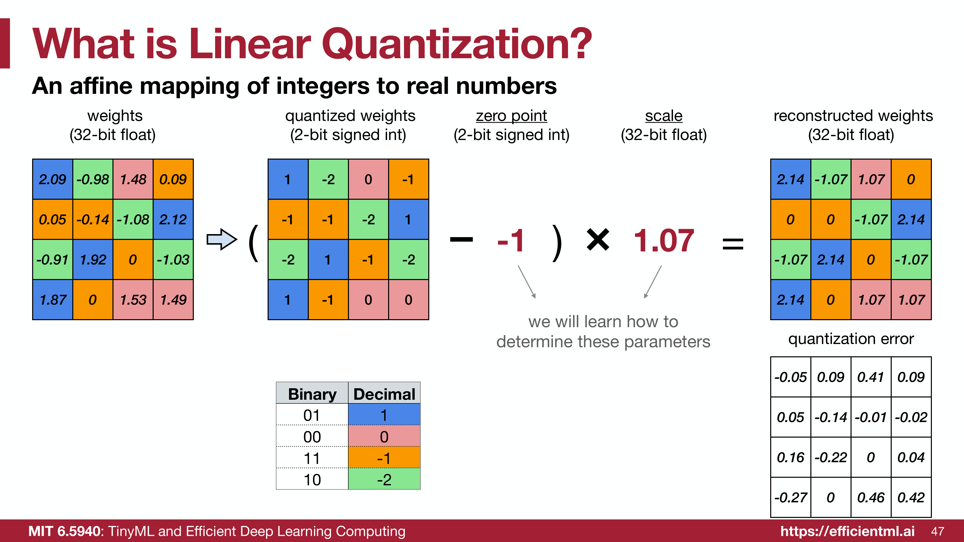 Affine mapping from integers to real numbers via scale and zero-point
Understanding the Components
The Scale Factor (S)
The scale factor determines the step size between consecutive integer values. A larger scale means coarser quantization with wider gaps between representable values.
For an N-bit quantization covering the range $[r_{\min}, r_{\max}]$:
\[S = \frac{r_{\max} - r_{\min}}{q_{\max} - q_{\min}}\]where $q_{\min} = -2^{N-1}$ and $q_{\max} = 2^{N-1} - 1$ for signed integers.
Example: Consider quantizing weights in range $[-1.08, 2.12]$ to 2-bit signed integers $[-2, 1]$:
\[S = \frac{2.12 - (-1.08)}{1 - (-2)} = \frac{3.20}{3} = 1.07\]This means consecutive integer values are separated by 1.07 in floating-point space.
The Zero Point (Z)
The zero point ensures that the floating-point value $r = 0$ can be represented exactly by an integer. This proves critical for handling padding in convolutional layers and maintaining numerical stability.
From the quantization formula $r = S(q - Z)$, setting $r = 0$ gives:
\[0 = S(q - Z) \implies q = Z\]We can derive the zero point from the range boundaries:
\[r_{\min} = S(q_{\min} - Z) \implies Z = q_{\min} - \frac{r_{\min}}{S}\]In practice, we round to the nearest integer:
\[Z = \text{round}\left(q_{\min} - \frac{r_{\min}}{S}\right)\]Continuing our example with $r_{\min} = -1.08$, $q_{\min} = -2$, and $S = 1.07$:
\[Z = \text{round}\left(-2 - \frac{-1.08}{1.07}\right) = \text{round}(-2 + 1.01) = -1\]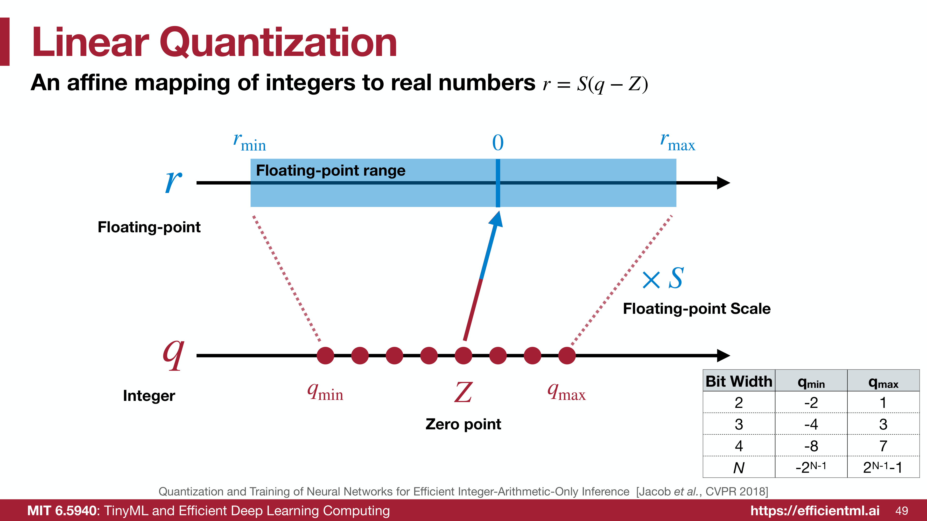 Visualization of scale, zero point, and the quantization mapping
The Quantization Process
Forward Quantization (FP32 → INT8)
To convert a real number $r$ to its quantized integer representation:
\[q = \text{round}\left(\frac{r}{S} + Z\right)\]We must also clip to ensure the result stays within representable range:
\[q = \text{clip}\left(\text{round}\left(\frac{r}{S} + Z\right), q_{\min}, q_{\max}\right)\]Example quantizing the weight matrix:
| Original Weight (r) | Computation | Quantized Value (q) |
|---|---|---|
| 2.09 | round(2.09/1.07 - 1) | 1 |
| -0.98 | round(-0.98/1.07 - 1) | -2 |
| 1.48 | round(1.48/1.07 - 1) | 0 |
| 0.09 | round(0.09/1.07 - 1) | -1 |
Dequantization (INT8 → FP32)
Recovery to floating-point uses the inverse transformation:
\[r = S(q - Z)\]This reconstruction introduces quantization error:
\[\epsilon = r_{\text{original}} - r_{\text{reconstructed}}\]The magnitude of this error depends on the scale factor—smaller scales mean higher precision but narrower range.
Symmetric vs Asymmetric Quantization
Linear quantization comes in two flavors, each with distinct trade-offs.
Asymmetric Quantization
The general form we’ve discussed allows arbitrary $Z$ values and asymmetric ranges. The floating-point range $[r_{\min}, r_{\max}]$ doesn’t need to be centered at zero.
Advantages:
- Full range utilization: Every integer value maps to the actual data range
- Flexibility: Adapts to skewed weight/activation distributions
- Optimal precision: Minimizes quantization error for asymmetric data
Disadvantages:
- Zero-point computation overhead: Requires addition/subtraction operations in the inference path
- More complex hardware: Needs extra logic for zero-point handling
Symmetric Quantization
| Sets $Z = 0$, forcing the floating-point range to be symmetric around zero: $[- | r | _{\max}, | r | _{\max}]$. |
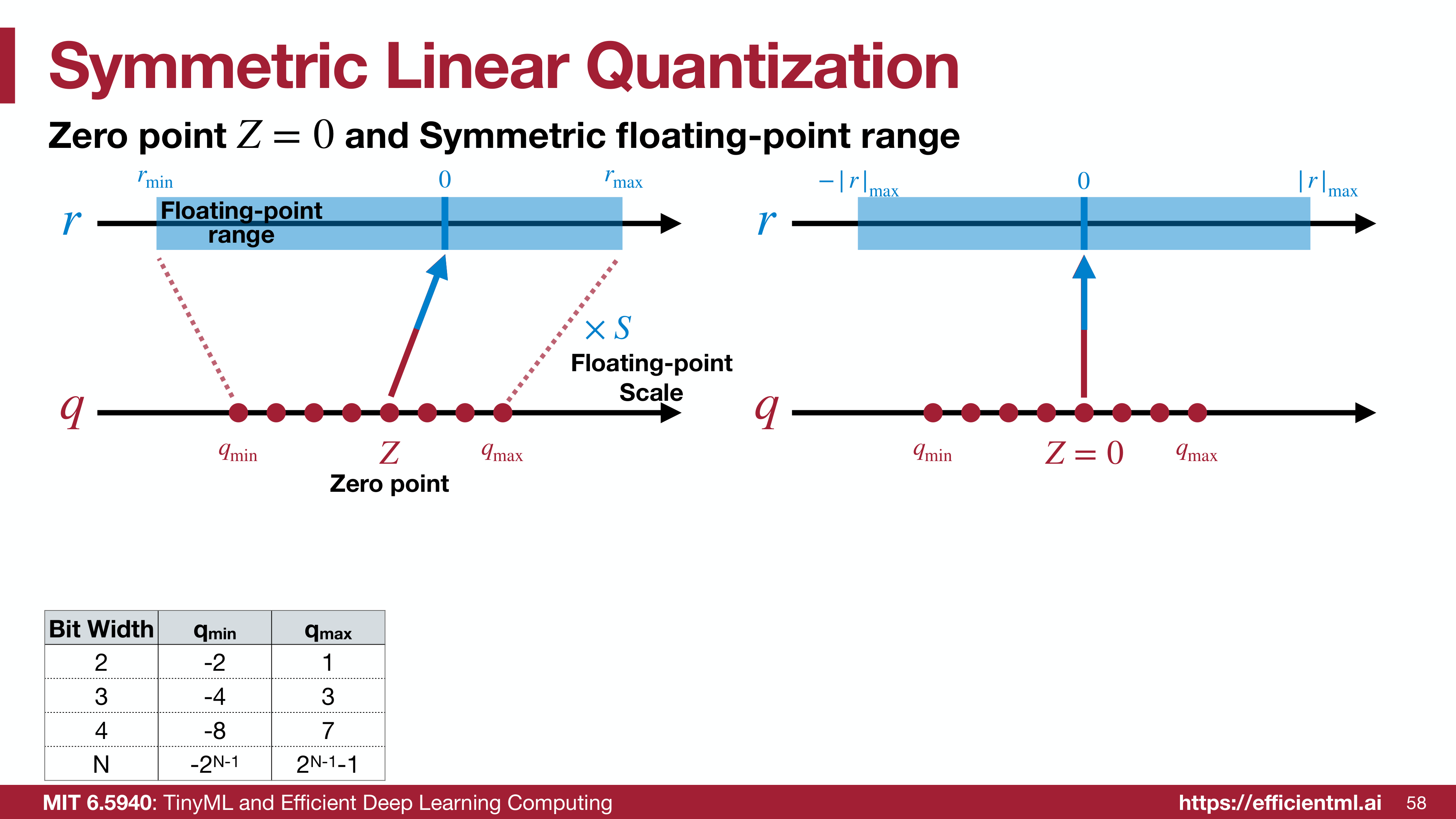 Symmetric quantization with zero point at origin
The scale factor becomes:
\[S = \frac{|r|_{\max}}{2^{N-1}}\]Full-range mode: Uses all available integer values:
\[S = \frac{|r|_{\max}}{2^{N-1}}\]For $N = 8$, this gives $q \in [-128, 127]$.
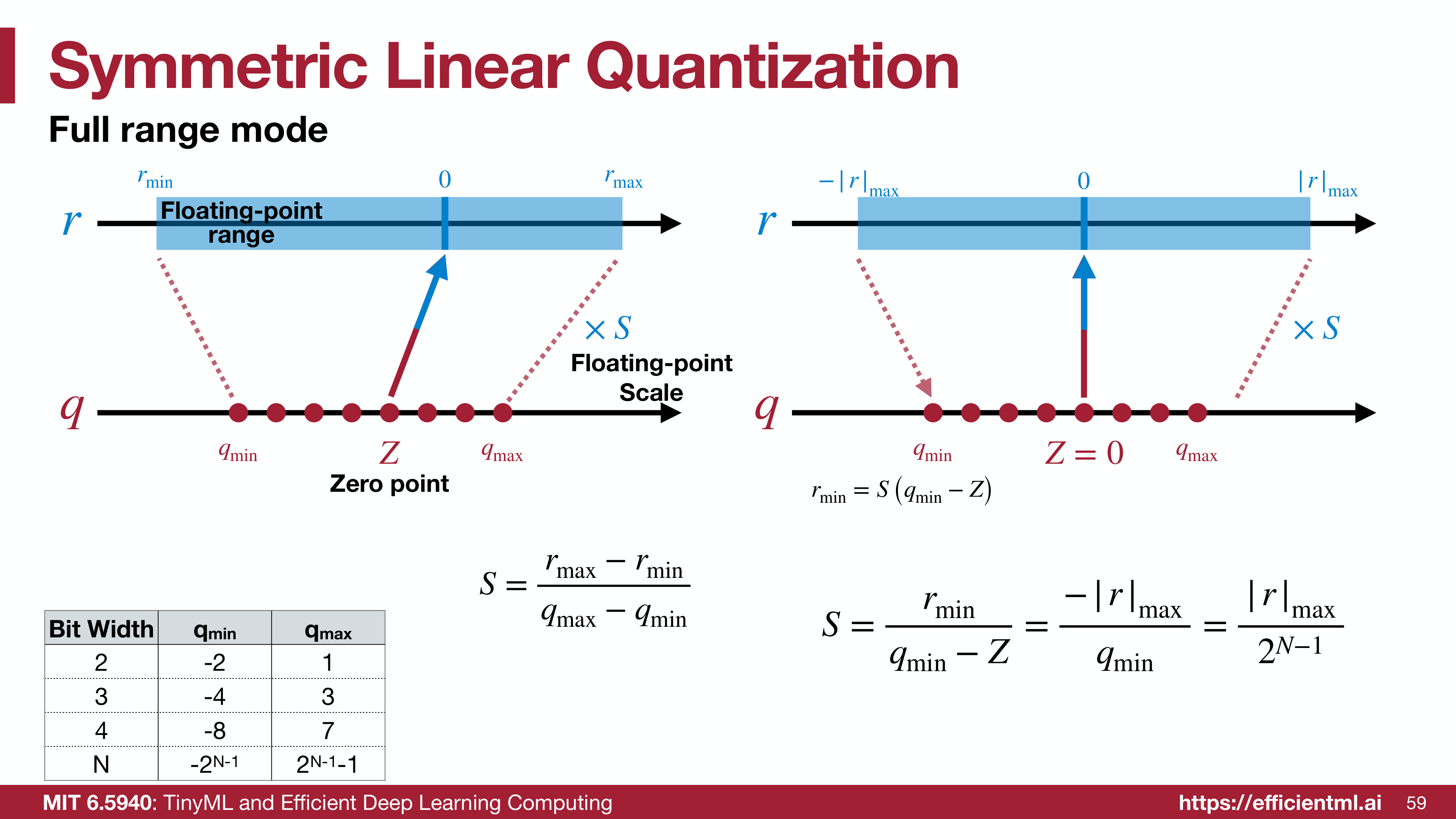 Scale factor calculation for symmetric quantization
Restricted-range mode: Excludes the minimum integer value to maintain perfect symmetry:
\[S = \frac{|r|_{\max}}{2^{N-1} - 1}\]For $N = 8$, this uses $q \in [-127, 127]$, sacrificing one representable value for mathematical convenience.
Advantages:
- Hardware efficiency: Eliminates zero-point arithmetic, simplifying hardware
- Faster inference: Fewer operations in the critical path
- Simpler implementation: Less complex quantization logic
Disadvantages:
- Range waste: When data is skewed (e.g., ReLU activations are non-negative), half the integer range represents values that never occur
- Lower precision: For asymmetric data, effective precision is reduced
Choosing the Right Mode
Use symmetric quantization when:
- Weights are roughly centered around zero (typically true for well-initialized networks)
- Hardware efficiency is paramount
- Implementing quantization-aware training
Use asymmetric quantization when:
- Data has significant skew (e.g., post-ReLU activations)
- Maximizing accuracy for post-training quantization
- Range utilization matters more than hardware efficiency
Per-Tensor vs Per-Channel Quantization
The granularity of quantization parameters significantly impacts accuracy.
Per-Tensor Quantization
Uses a single scale factor and zero point for the entire weight tensor or activation tensor.
For a weight tensor $W$ of shape $[C_{\text{out}}, C_{\text{in}}, K_h, K_w]$:
\[S_W = \frac{\max(W) - \min(W)}{q_{\max} - q_{\min}}\] \[Z_W = \text{round}\left(q_{\min} - \frac{\min(W)}{S_W}\right)\]Advantages:
- Simple implementation
- Minimal memory overhead
- Fast execution
Disadvantages:
- Poor accuracy when tensor has wide dynamic range across channels
- Outliers in one channel affect quantization quality of all channels
Per-Channel Quantization
Uses separate scale factors (and zero points) for each output channel.
For each output channel $i$:
\[S_{W,i} = \frac{\max(W[i, :, :, :]) - \min(W[i, :, :, :])}{q_{\max} - q_{\min}}\]Advantages:
- Better accuracy: Adapts to per-channel statistics
- Handles outliers: Extreme values in one channel don’t affect others
- Minimal overhead: Scale factors stored once per channel
Disadvantages:
- Slightly more complex implementation
- Small memory overhead (typically negligible)
Practical recommendation: Always use per-channel quantization for weights. The accuracy improvement vastly outweighs the minimal overhead. For activations, per-tensor quantization usually suffices since activations tend to have more uniform distributions within a layer.
Determining Quantization Parameters
Calibration Process
For post-training quantization, we need to determine optimal scale and zero-point without retraining.
Step 1: Collect statistics by running inference on a calibration dataset (typically 100-1000 samples):
\(r_{\min} = \min(\text{weights or activations})\) \(r_{\max} = \max(\text{weights or activations})\)
Step 2: Compute scale and zero point using the formulas:
\[S = \frac{r_{\max} - r_{\min}}{q_{\max} - q_{\min}}\] \[Z = \text{round}\left(q_{\min} - \frac{r_{\min}}{S}\right)\]Step 3: Validate on a validation set and adjust if accuracy degrades significantly.
Handling Outliers
Outliers can drastically increase the scale factor, reducing effective precision. Several strategies mitigate this:
Percentile-based clipping: Use 99.9th percentile instead of absolute maximum:
\(r_{\max} = \text{percentile}(r, 99.9)\) \(r_{\min} = \text{percentile}(r, 0.1)\)
KL divergence minimization: Find clipping threshold that minimizes information loss between original and quantized distributions.
Moving average: For activations during training, maintain exponential moving average of min/max values:
\[r_{\max}^{(t)} = \alpha \cdot r_{\max}^{(t-1)} + (1-\alpha) \cdot \max(r^{(t)})\]Quantization-Aware Training
For maximum accuracy, incorporate quantization into the training process itself.
Fake Quantization
During training, simulate quantization effects while keeping everything in floating-point:
\[\tilde{w} = S \cdot \text{round}\left(\frac{w}{S} + Z\right) - Z \cdot S\]This “fake quantization” node is differentiable (using straight-through estimator for gradients) and allows the network to learn weights that tolerate quantization.
Straight-Through Estimator (STE)
The rounding operation is non-differentiable. STE approximates the gradient:
\[\frac{\partial \text{round}(x)}{\partial x} \approx 1 \quad \text{(treat as identity)}\]This allows gradients to flow through the quantization node during backpropagation, enabling end-to-end training.
Training Recipe
- Start from pretrained model: Begin with full-precision weights
- Insert fake quantization: Add quantization simulation to forward pass
- Fine-tune: Train for 10-20% of original training epochs
- Use lower learning rate: Typically 1/10th of initial training rate
- Gradual freezing: Progressively freeze layers starting from input
Mathematical Properties and Optimizations
Scale Factor Representation
In practice, the scale factor $S$ can be represented efficiently. Empirically, $S_W \cdot S_X / S_Y$ (the combined scale for a layer) falls in $(0, 1)$ and can be expressed as:
\[\frac{S_W \cdot S_X}{S_Y} = 2^{-n} \cdot M_0, \quad M_0 \in [0.5, 1)\]This representation enables efficient fixed-point multiplication followed by bit-shift:
\[q_Y = (M_0 \cdot \text{temp}) \gg n\]where >> is right-shift. This avoids expensive floating-point operations during inference.
Fusing Scale Factors
For layers without activation functions, scale factors can be fused:
\[Y = W \cdot X \implies S_Y(q_Y - Z_Y) = S_W(q_W - Z_W) \cdot S_X(q_X - Z_X)\]Rearranging:
\[q_Y = \frac{S_W \cdot S_X}{S_Y}(q_W - Z_W)(q_X - Z_X) + Z_Y\]The combined scale $S_W \cdot S_X / S_Y$ can be precomputed and baked into the model, reducing runtime overhead.
Practical Considerations
Layer-Specific Strategies
First layer: Often kept in FP16 or FP32 since it directly processes input data, which may have wide dynamic range.
Last layer: Classification layers are sensitive to quantization. Consider 8-bit instead of 4-bit.
Batch normalization: Fold BN parameters into preceding convolution to eliminate BN overhead:
\[y = \gamma \cdot \frac{x - \mu}{\sqrt{\sigma^2 + \epsilon}} + \beta\]This can be absorbed into $W$ and $b$ of the convolution layer.
Activation Functions
ReLU: Perfectly compatible with linear quantization. For post-ReLU activations, $r_{\min} = 0$, allowing asymmetric quantization with full range utilization.
Non-monotonic functions (Swish, GELU): More challenging to quantize. May require higher precision or piecewise linear approximation.
Hardware Mapping
Modern hardware (ARM NEON, Intel VNNI, NVIDIA Tensor Cores) includes specialized instructions for:
- INT8 × INT8 → INT32 multiplication
- INT32 accumulation
- Efficient requantization (scale/shift operations)
Ensuring your quantization scheme maps to these instructions is critical for realizing speedups.
Accuracy Considerations
INT8 vs INT4
INT8 quantization:
- Typically maintains within 1% accuracy of FP32
- Widely supported in hardware
- Suitable for most production deployments
INT4 quantization:
- More aggressive, 2-4% accuracy degradation typical
- Requires careful per-channel quantization and calibration
- May need mixed-precision (some layers INT8, others INT4)
Calibration Dataset Size
Larger calibration sets improve quantization parameter estimation:
- 100 samples: Minimal baseline
- 500 samples: Good balance for most tasks
- 1000+ samples: Diminishing returns beyond this
Quantization-Aware Training Benefits
QAT typically recovers 50-90% of quantization error compared to post-training quantization:
| Method | INT8 Accuracy Drop | INT4 Accuracy Drop |
|---|---|---|
| Post-Training | 0.5-2% | 3-6% |
| QAT | 0.1-0.5% | 1-2% |
The improvement comes from the network learning to adapt its weights to be quantization-friendly.
Key Takeaways
- Linear quantization enables integer arithmetic via affine mapping: $r = S(q - Z)$
- Scale factor determines precision; zero point ensures exact representation of 0
- Symmetric quantization ($Z = 0$) simplifies hardware but wastes range for skewed data
- Per-channel quantization dramatically improves accuracy with minimal overhead
- Calibration determines quantization parameters from representative data
- Quantization-aware training adapts weights to tolerate quantization, recovering most accuracy
- Hardware efficiency comes from eliminating floating-point operations during inference
- Mixed-precision strategies balance accuracy and efficiency by using different bit-widths for different layers
Bridging to Inference
We’ve established the mathematical framework for linear quantization, but a critical question remains: how do we actually perform matrix multiplications, convolutions, and other neural network operations entirely in integer arithmetic?
Part 4 will complete the picture by deriving the quantized forms of these operations. We’ll see how to fuse bias addition, handle activation functions, and optimize the inference pipeline for maximum hardware efficiency—transforming theory into practical, deployable implementations.
Series Navigation:
- Part 1: Understanding Numeric Data Types
- Part 2: K-Means Based Weight Quantization
- Part 3: Linear Quantization Methods (Current)
- Part 4: Quantized Neural Network Operations
- Part 5: Post-Training Quantization Techniques
- Part 6: Quantization-Aware Training
- Part 7: Binary and Ternary Quantization
- Part 8: Mixed-Precision Quantization
References:
- MIT 6.5940: TinyML and Efficient Deep Learning Computing - EfficientML.ai Lecture 05: Quantization Part I (Fall 2024)
- Quantization and Training of Neural Networks for Efficient Integer-Arithmetic-Only Inference - Jacob et al., CVPR 2018
- Integer Quantization for Deep Learning Inference: Principles and Empirical Evaluation - Wu et al., 2020
- Neural Network Distiller: Linear Quantization