Quantization Part 7: Binary and Ternary Quantization

We’ve explored 8-bit and 4-bit quantization, achieving impressive efficiency with manageable accuracy trade-offs. But what if we push to the absolute extreme—representing weights with just a single bit? This is the realm of binary and ternary quantization, where weights take only two or three distinct values. The result? Elimination of expensive multiplications in favor of simple bit operations and additions, enabling unprecedented speed and energy efficiency. The cost? Significant accuracy degradation that requires careful mitigation strategies.

The Motivation for Extreme Quantization

Consider the computational breakdown in a typical neural network inference:

Standard FP32 convolution:

• Each multiply-accumulate (MAC): ~4 pJ energy
• Memory access for 32-bit weight: ~640 pJ (DRAM)
• Bottleneck: Memory access dominates (160× more energy than compute)

INT8 quantization:

• MAC energy: ~0.2 pJ (20× improvement)
• Memory access: ~160 pJ (4× improvement)
• Good but memory still bottleneck

Binary quantization:

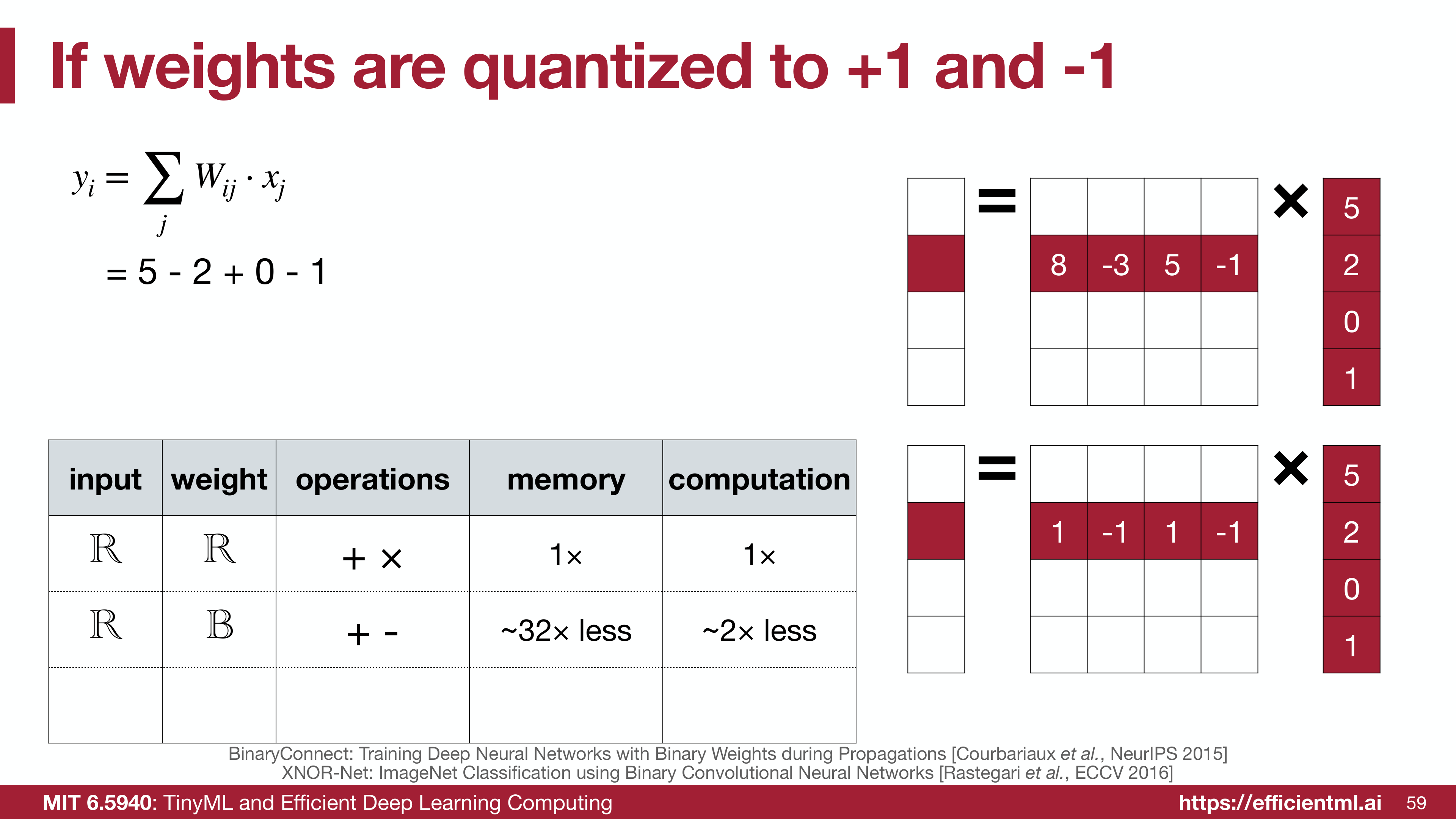
• No multiplications—only XNOR + popcount operations
• Memory access: ~20 pJ (32× improvement over FP32)
• Game-changer: Memory becomes manageable

Energy cost breakdown: 32-bit float vs 8-bit int vs 1-bit binary operations

The energy savings are dramatic:

• Memory access: 32× reduction (32 bits → 1 bit)
• Computation: 100× reduction (multiply → XNOR)
• Overall system energy: 10-50× improvement depending on model

But this comes at a steep price: typical accuracy drop of 5-15% on ImageNet classification.

Binary Quantization Fundamentals

The Basic Idea

Binary quantization constrains weights to just two values:

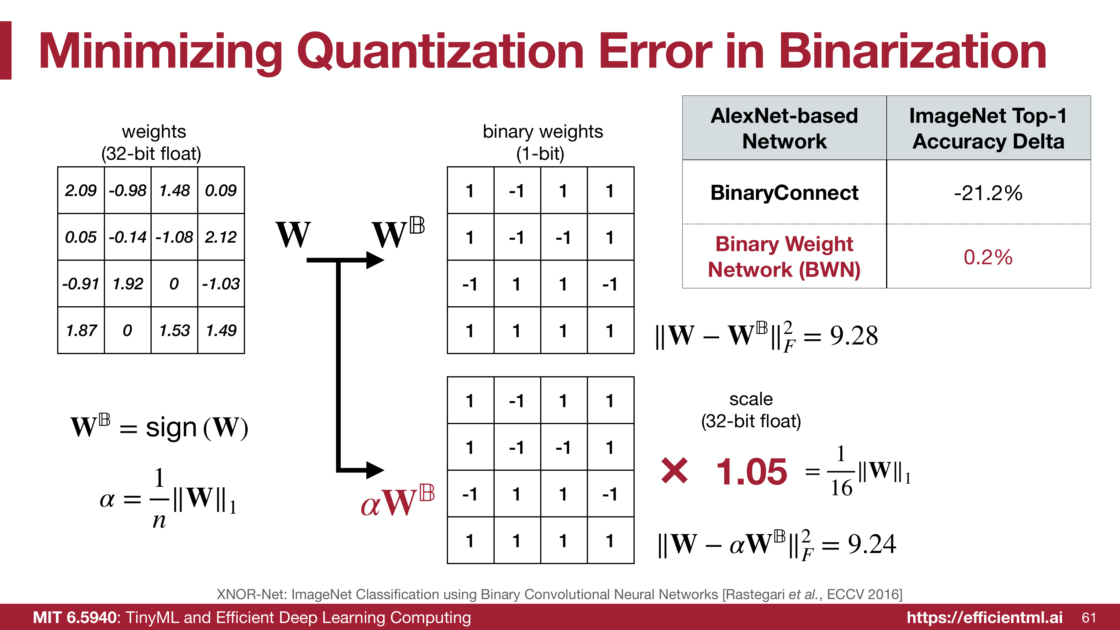
\[W_b \in \{-\alpha, +\alpha\}\]

where $\alpha$ is a scaling factor.

The simplest binarization uses the sign function:

\[W_b = \alpha \cdot \text{sign}(W)\]

where:

\[\text{sign}(W) = \begin{cases} +1 & \text{if } W \geq 0 \\ -1 & \text{if } W < 0 \end{cases}\]

Key insight: Each weight becomes a single bit (+ or −), reducing memory footprint by 32×.

Computing the Scale Factor

To minimize quantization error, we choose $\alpha$ to minimize:

\[\| W - W_b \|_2^2 = \| W - \alpha \cdot \text{sign}(W) \|_2^2\]

Taking the derivative and setting to zero:

\[\frac{\partial}{\partial \alpha} \| W - \alpha \cdot \text{sign}(W) \|_2^2 = 0\]

This yields the optimal scale:

\[\alpha^* = \frac{1}{n} \sum_{i=1}^{n} |W_i| = \mathbb{E}[|W|]\]

Interpretation: The scaling factor is simply the mean absolute value of weights—this minimizes the $L^2$ reconstruction error.

BinaryConnect: The First Practical Binary Network

BinaryConnect (Courbariaux et al., 2015) introduced a training procedure for binary weights:

Forward pass:

\[W_b = \text{sign}(W_{\text{real}})\] \[Y = X \cdot W_b\]

Backward pass:

\[\frac{\partial L}{\partial W_{\text{real}}} = \frac{\partial L}{\partial W_b} \cdot \underbrace{\frac{\partial W_b}{\partial W_{\text{real}}}}_{\text{STE: } = 1}\]

Weight update:

\[W_{\text{real}} \leftarrow W_{\text{real}} - \eta \cdot \frac{\partial L}{\partial W_{\text{real}}}\]

Critical observation: Real-valued weights $W_{\text{real}}$ are maintained during training and updated by gradients, but only binary weights $W_b$ are used in the forward pass.

This dual-representation strategy (similar to QAT in Part 6) allows gradients to accumulate small changes in $W_{\text{real}}$ that eventually flip the sign of $W_b$.

BinaryConnect maintains full-precision weights during training, binarizes for forward pass

Binary Weight Networks (BWN)

Binary Weight Networks (Rastegari et al., 2016) improved upon BinaryConnect by introducing:

1. Per-channel scaling factors: Instead of global $\alpha$, compute $\alpha_i$ per filter:

\[\alpha_i = \frac{1}{c \cdot k \cdot k} \sum_{c,k,k} |W_{i,c,k,k}|\]

2. Efficient binarization: Store weights as bit arrays for 32× memory compression

3. Binary matrix multiplication: Replace $Y = X \cdot W$ with efficient binary operations

Implementation Details

Binarization:

def binarize_weights(W):
    # Compute per-filter scale factors
    alpha = W.abs().mean(dim=[1,2,3], keepdim=True)
    
    # Binarize
    W_binary = alpha * torch.sign(W)
    
    return W_binary, alpha

Storage:

# Pack 32 binary weights into single 32-bit integer
def pack_binary_weights(W_binary):
    # W_binary: [out_ch, in_ch, k, k] with values {-1, +1}
    W_bits = (W_binary > 0).to(torch.uint8)  # Convert to {0, 1}
    
    # Pack 32 weights per integer
    W_packed = torch.zeros(out_ch, in_ch // 32, k, k, dtype=torch.int32)
    for i in range(32):
        W_packed += W_bits[:, i::32, :, :] << i
    
    return W_packed

Accuracy on ImageNet (AlexNet):

Method	Top-1 Accuracy	Memory	Speedup
FP32 Baseline	56.6%	233 MB	1×
Binary Weights	50.1%	7.3 MB	3.4×

Analysis: 6.5% accuracy drop, but 32× memory reduction and 3.4× speedup.

XNOR-Net: Binary Weights AND Activations

BWN binarizes only weights, keeping activations in full precision. XNOR-Net takes the next step: binarize both weights and activations.

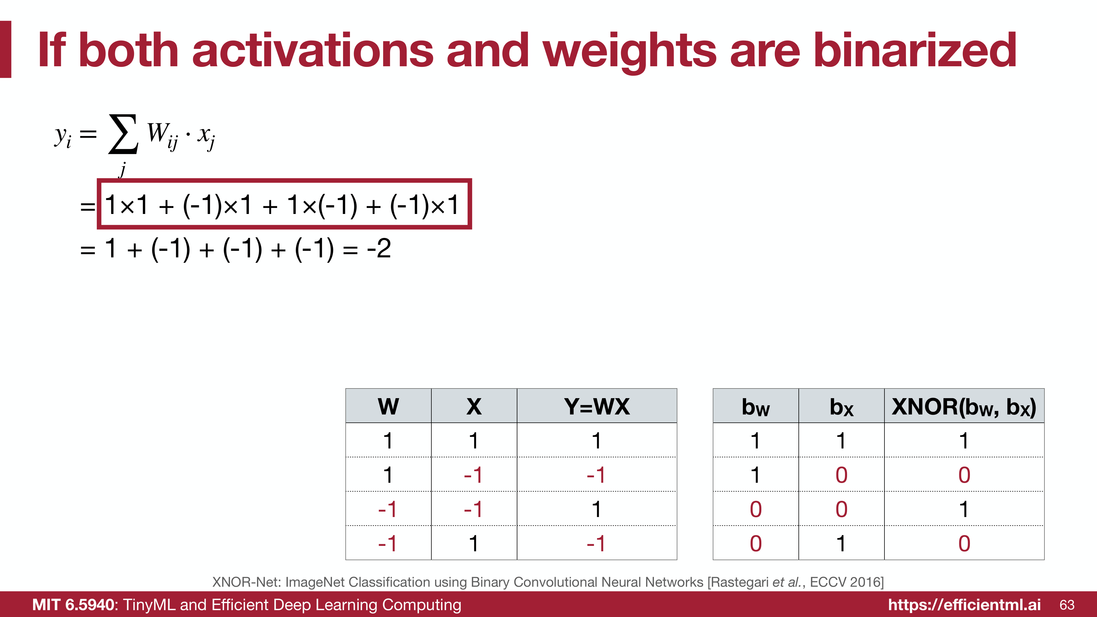XNOR-Net binarizes both weights and activations for maximum efficiency

The XNOR Operation

When both inputs are binary, matrix multiplication reduces to:

\[Y = (X_b \odot W_b) \cdot \alpha_X \cdot \alpha_W\]

where $\odot$ is element-wise XNOR:

\[\text{XNOR}(a, b) = \begin{cases} 1 & \text{if } a = b \\ 0 & \text{if } a \neq b \end{cases}\]

Key insight:

\[\text{XNOR}(a, b) = 1 - \text{XOR}(a, b)\]

So the inner product becomes:

\[\langle X_b, W_b \rangle = \sum_{i} \text{XNOR}(X_b^i, W_b^i) = n - \sum_{i} \text{XOR}(X_b^i, W_b^i)\]

Efficient Implementation

Modern CPUs/GPUs have specialized instructions:

CPU (x86):

// XNOR 64 bits at once
uint64_t xnor_result = ~(x_binary ^ w_binary);

// Count 1s (popcount)
int dot_product = __builtin_popcountll(xnor_result);

GPU (CUDA):

// XNOR 32 weights simultaneously
uint32_t xnor = ~(x_binary ^ w_binary);

// Count bits using __popc intrinsic
int dot_product = __popc(xnor);

This replaces:

• 32 multiplications + 32 additions
• With 1 XNOR + 1 popcount

Speedup: 60-100× in binary computation alone.

Scaling Factor Computation

For activations, compute per-spatial-location scales:

\[\alpha_X^{(i,j)} = \frac{1}{c} \sum_{c} |X_{c,i,j}|\]

For weights, per-channel scales:

\[\alpha_W^{(k)} = \frac{1}{c \cdot h \cdot w} \sum |W_{k,c,h,w}|\]

The output is then:

\[Y = (X_b \odot W_b) \cdot \alpha_X \cdot \alpha_W\]

where scaling factors are applied after binary convolution.

XNOR-Net Results

ImageNet (AlexNet):

Network	Top-1 Accuracy	Memory	Compute
FP32 Baseline	56.6%	233 MB	1.0×
Binary Weights (BWN)	50.1%	7.3 MB	3.4×
Binary Weights + Activations (XNOR)	44.2%	7.3 MB	58×

Critical trade-off: 12.4% accuracy drop for 58× compute speedup.

Where XNOR-Net Works Well

Object detection (Pascal VOC):

• Faster R-CNN with XNOR-Net backbone
• 56.8 mAP (FP32) → 51.5 mAP (XNOR)
• Only 5.3 mAP drop (less than classification!)

Semantic segmentation:

• Binary FCN for real-time segmentation
• 30 FPS on embedded devices

Why better for detection/segmentation?

• Spatial features more robust to quantization
• Lower-level features (edges, textures) preserved better than high-level semantics

Ternary Quantization: Adding Zero

Binary quantization is aggressive—every weight contributes equally to the computation. Ternary quantization introduces a third value: zero.

\[W_t \in \{-\alpha, 0, +\alpha\}\]

Motivation: Allow the network to explicitly suppress less important connections by setting weights to zero, creating structured sparsity.

Ternary Weight Networks (TWN)

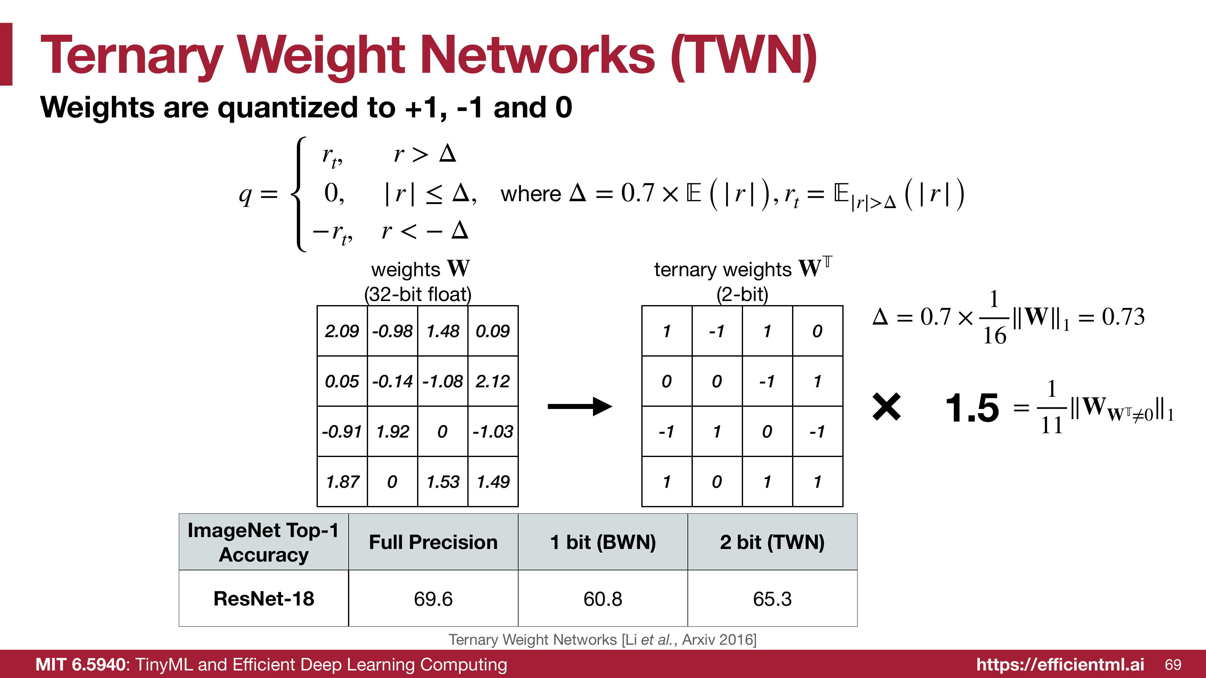
TWN (Li et al., 2016) uses a threshold-based ternization:

\[W_t = \begin{cases} +\alpha & \text{if } W > \Delta \\ 0 & \text{if } |W| \leq \Delta \\ -\alpha & \text{if } W < -\Delta \end{cases}\]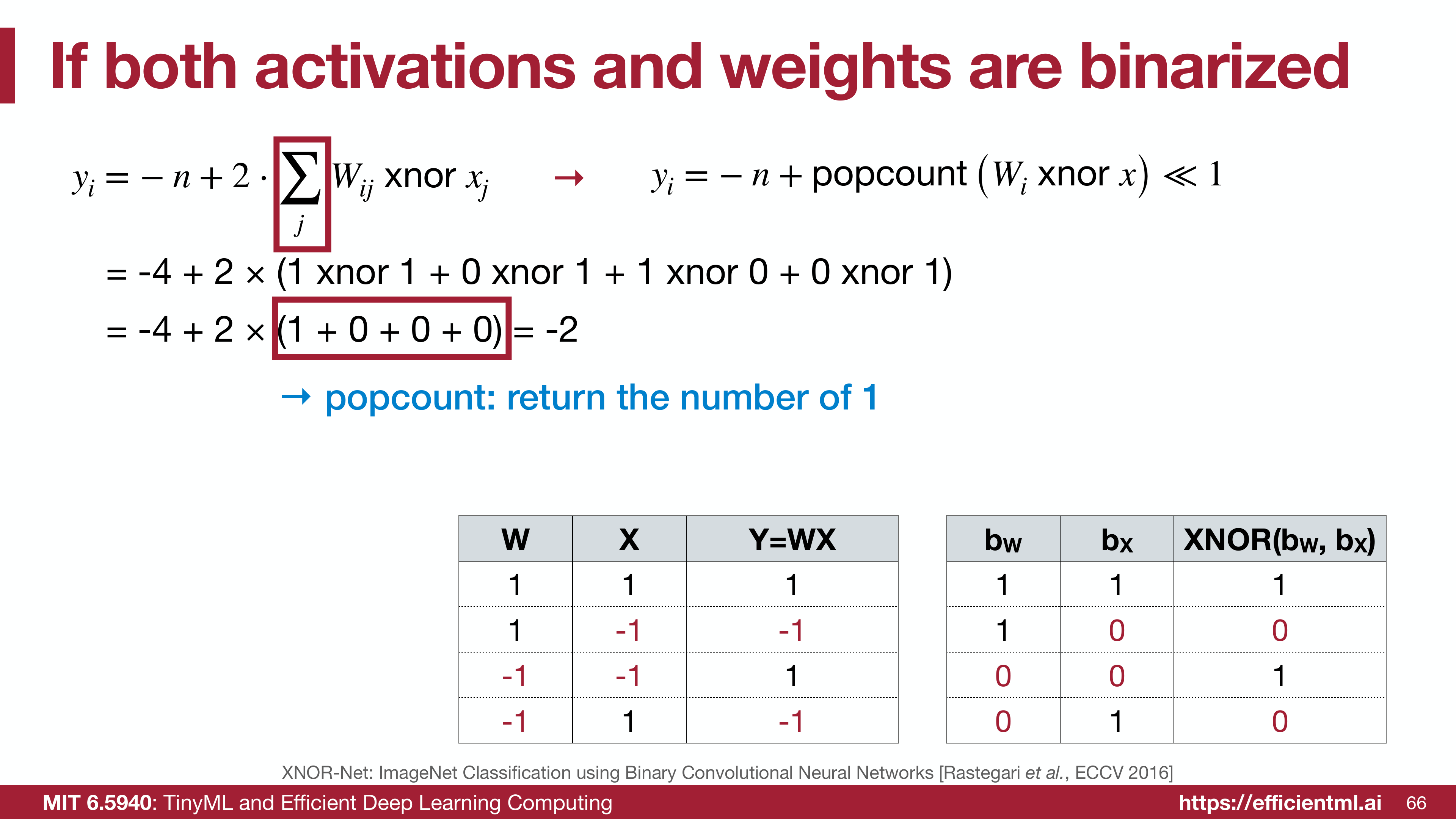

Ternary quantization introduces zero threshold for structured sparsity

Optimal threshold: Minimize quantization error:

\[\Delta^* = \frac{0.7}{n} \sum_{i=1}^{n} |W_i|\]

Scaling factor:

\[\alpha^* = \frac{\sum_{|W_i| > \Delta} |W_i|}{\sum_{|W_i| > \Delta} 1}\]

Interpretation:

• $\alpha$ is the mean magnitude of weights that survive the threshold
• $\Delta$ is set to suppress ~30-40% of weights with smallest magnitude

Storage and Computation

Memory: Ternary values need 2 bits (00 = 0, 01 = +1, 11 = -1)

• 16× memory reduction vs FP32

Computation: Skip multiplications for zero weights

• If 40% weights are zero, 40% fewer operations
• Remaining operations still use $\pm \alpha$ scaling

Effective speedup: 5-10× depending on sparsity and hardware support.

Trained Ternary Quantization (TTQ)

TTQ (Zhu et al., 2017) makes the ternary values learnable rather than fixed:

\[W_t \in \{-W_p, 0, W_n\}\]

where $W_p > 0$ and $W_n > 0$ are positive and negative scale factors, learned during training.

TTQ learns asymmetric positive and negative scales

Why Asymmetric Scales?

In many layers, weight distributions are asymmetric:

ReLU layers: Positive weights may be more important (forward signal propagation)

Residual connections: Negative weights critical for identity mapping

TTQ adapts $W_p$ and $W_n$ independently to capture this asymmetry.

TTQ Training Procedure

Quantization function:

\[W_t = \begin{cases} W_p & \text{if } W > \Delta \\ 0 & \text{if } |W| \leq \Delta \\ -W_n & \text{if } W < -\Delta \end{cases}\]

Gradient updates (using STE):

\[\frac{\partial L}{\partial W_p} = \sum_{W_i > \Delta} \frac{\partial L}{\partial W_{t,i}}\] \[\frac{\partial L}{\partial W_n} = \sum_{W_i < -\Delta} \frac{\partial L}{\partial W_{t,i}}\]

Both $W_p$ and $W_n$ are optimized alongside the ternization threshold $\Delta$.

TTQ Results

ResNet-18 on ImageNet:

Method	Top-1 Accuracy	Bit-width	Memory
FP32 Baseline	69.6%	32	46 MB
TWN (symmetric)	65.3%	2	2.9 MB
TTQ (asymmetric)	66.6%	2	2.9 MB

Observation: Learning asymmetric scales recovers 1.3% accuracy over fixed symmetric scales—a significant improvement in the ultra-low precision regime.

Gradient Computation for Binary/Ternary

The non-differentiability of sign() and threshold functions requires careful gradient handling.

Straight-Through Estimator Variants

Standard STE (used in BinaryConnect):

\[\frac{\partial \text{sign}(W)}{\partial W} = 1\]

Clipped STE:

\[\frac{\partial \text{sign}(W)}{\partial W} = \begin{cases} 1 & \text{if } |W| \leq 1 \\ 0 & \text{otherwise} \end{cases}\]

Rationale: Only update weights close to decision boundary (where gradient is meaningful).

Swish-sign (smooth approximation):

\[\text{sign}_{\text{smooth}}(W) = \tanh(\beta \cdot W)\]

where $\beta$ controls steepness. As $\beta \to \infty$, $\tanh(\beta W) \to \text{sign}(W)$.

During training, use smooth version for gradients:

\[\frac{\partial \text{sign}_{\text{smooth}}(W)}{\partial W} = \beta \cdot \text{sech}^2(\beta W)\]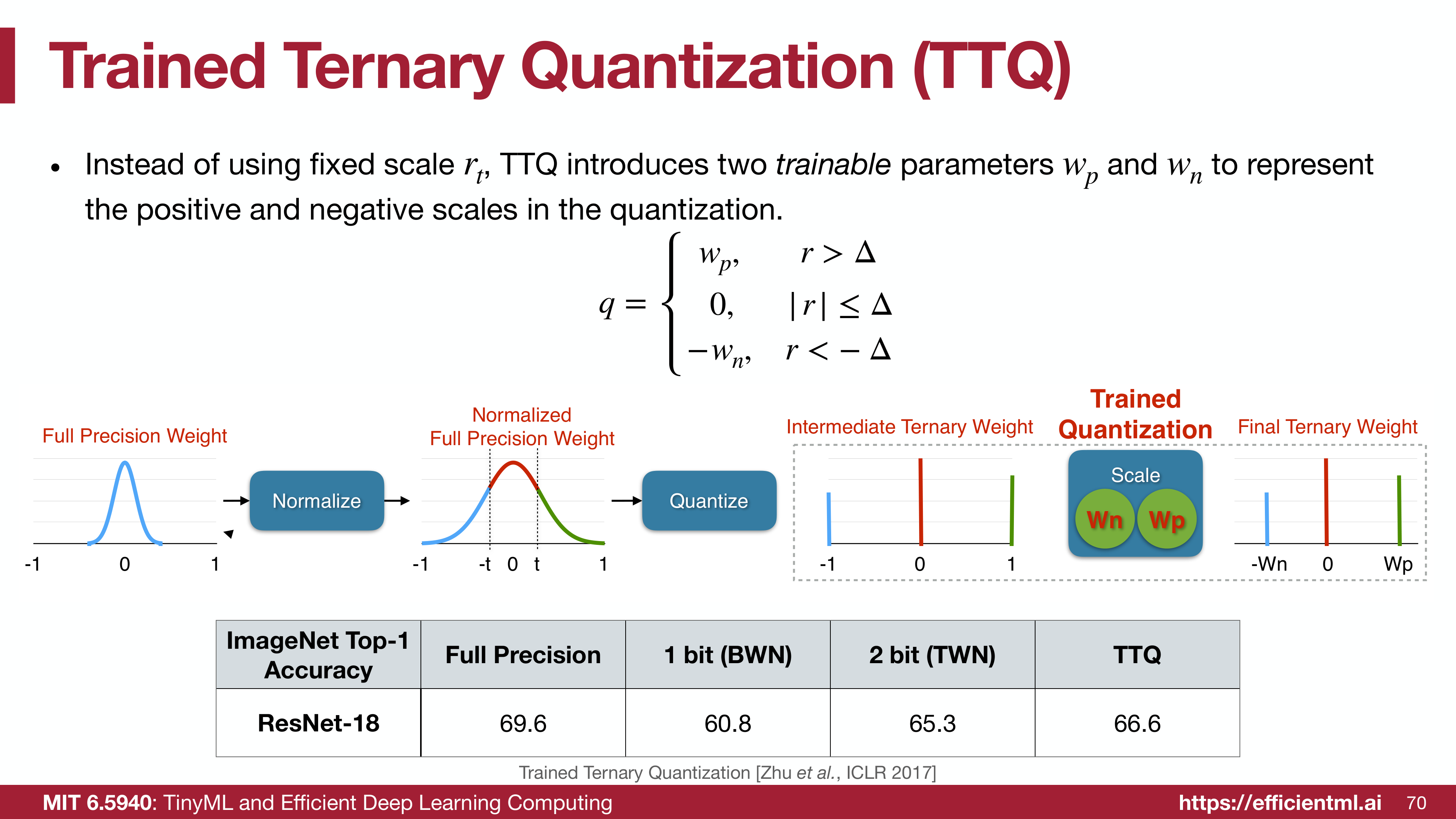

Different STE variants for binary quantization

Which STE to Use?

Standard STE: Simple, works well for most cases

Clipped STE: Better for extreme quantization (1-2 bit)

Swish-sign: Smoothest training, best for small models

Empirical finding: Choice of STE matters less than proper learning rate and training schedule.

Practical Training Strategies

Training from Scratch vs Fine-Tuning

From scratch:

• Use higher initial learning rate (0.1-0.01)
• Longer training (300-500 epochs)
• Heavy data augmentation essential

Fine-tuning from FP32:

• Lower learning rate (0.001-0.0001)
• Shorter training (50-100 epochs)
• Usually achieves better accuracy

Recommendation: Always start with FP32 pretrained model for binary/ternary quantization.

Layer-wise Strategies

Keep first and last layers in higher precision:

# First conv: FP32 or INT8
model.conv1.quantize = False

# Middle layers: Binary/Ternary
for layer in model.middle_layers:
    layer.quantize = True
    layer.bit_width = 1  # or 2 for ternary

# Classifier: FP32 or INT8
model.fc.quantize = False

Rationale:

• First layer: input features need fine-grained representation
• Last layer: class boundaries sensitive to quantization

Batch Normalization

Critical for binary networks: BN stabilizes training by normalizing activations before binarization.

Best practice:

# Order matters!
x = conv_binary(x)
x = batch_norm(x)  # Before activation binarization
x = binarize_activation(x)

BN reduces internal covariate shift caused by aggressive quantization.

Hardware Efficiency Analysis

Memory Bandwidth Savings

AlexNet example:

• Total parameters: 61M weights
• FP32: 61M × 4 bytes = 244 MB
• Binary: 61M × 1 bit = 7.6 MB
• 32× reduction

Memory access time (DRAM):

• FP32: 244 MB / 10 GB/s = 24.4 ms
• Binary: 7.6 MB / 10 GB/s = 0.76 ms
• 32× faster

Compute Efficiency

Single MAC operation:

• FP32 multiply: 3.7 pJ
• FP32 add: 0.9 pJ
• Total FP32 MAC: 4.6 pJ

Binary operation:

• XNOR: 0.05 pJ
• Popcount: 0.1 pJ
• Total binary MAC: 0.15 pJ

Energy reduction: 30× per operation

End-to-End System Impact

For AlexNet inference on mobile device:

Network	Energy (mJ)	Latency (ms)	Power (W)
FP32	420	95	4.4
INT8	105	38	2.8
Binary	21	12	1.8

Real-world speedup: 8× over FP32, 3× over INT8.

When to Use Binary/Ternary Quantization

Use Cases Where It Works

1. Embedded vision (object detection, tracking):

• Real-time requirements (>30 FPS)
• Power-constrained devices
• Small models (MobileNet-scale)

2. Keyword spotting:

• Binary RNNs for audio processing
• Always-on listening with <1 mW power

3. Recommendation systems:

• Binary embeddings for fast similarity search
• 100× speedup in dot product computation

When to Avoid

1. Large-scale classification:

• ImageNet Top-1 accuracy drops too much (10-15%)
• Better to use INT4 or mixed-precision

2. Generative models:

• GANs, diffusion models need fine-grained distributions
• Binary quantization destroys sample quality

3. When accuracy is critical:

• Medical imaging, autonomous driving
• Safety-critical applications

Accuracy Recovery Techniques

1. Knowledge Distillation

Train binary student network using FP32 teacher:

\[L_{\text{total}} = L_{\text{CE}}(y_{\text{student}}, y_{\text{true}}) + \lambda \cdot L_{\text{KD}}(y_{\text{student}}, y_{\text{teacher}})\]

Typical improvement: 2-3% accuracy recovery.

2. Wider Networks

Compensate for reduced representational capacity:

• FP32 ResNet-18: 69.6% accuracy
• Binary ResNet-18: 55.2% accuracy
• Binary ResNet-34 (2× wider): 61.3% accuracy

Trade-off: More parameters but still 16-32× memory savings.

3. Hybrid Precision

Use higher precision for sensitive layers:

# 1st conv, last FC: INT8
# All other layers: Binary

# Achieves better accuracy-efficiency trade-off

4. Dense-Sparse-Dense (DSD) Training

1. Dense: Train full-precision network
2. Sparse: Prune and binarize
3. Dense: Fine-tune with expanded capacity

This 3-stage approach recovers significant accuracy.

Key Takeaways

• Binary quantization: Weights in {-1, +1}, 32× memory reduction, 30-60× compute speedup
• XNOR-Net: Binarizes both weights and activations, replaces multiplications with XNOR+popcount operations
• Ternary quantization: Adds zero value for structured sparsity, 16× memory reduction
• TTQ: Learns asymmetric positive and negative scales, improving accuracy over fixed scales
• Gradient flow: Requires Straight-Through Estimator variants (standard, clipped, smooth)
• Training strategy: Fine-tuning from FP32 pretrained models works better than training from scratch
• Layer-wise precision: Keep first/last layers in higher precision (FP32 or INT8)
• Accuracy cost: Typically 5-15% drop on ImageNet, less severe for detection/segmentation tasks
• Best use cases: Embedded vision, keyword spotting, recommendation systems where speed/power critical
• Hardware efficiency: 32× memory bandwidth savings, 30× energy per operation, 8× end-to-end speedup

Bridging to Mixed Precision

Binary and ternary quantization demonstrate that not all layers need the same precision. Some layers tolerate 1-bit weights; others require 8 bits to maintain accuracy. This observation leads naturally to mixed-precision quantization, where bit-widths are assigned per-layer based on sensitivity.

Part 8 explores HAQ (Hardware-Aware Automated Quantization), which uses reinforcement learning to automatically search for optimal per-layer bit-widths while respecting hardware constraints like memory, latency, and energy budgets. Instead of uniform quantization or manual layer selection, HAQ learns a precision policy that maximizes accuracy under strict resource constraints.

---

Series Navigation:

• Part 1: Understanding Numeric Data Types
• Part 2: K-Means Based Weight Quantization
• Part 3: Linear Quantization Methods
• Part 4: Quantized Neural Network Operations
• Part 5: Post-Training Quantization Techniques
• Part 6: Quantization-Aware Training
• Part 7: Binary and Ternary Quantization (Current)
• Part 8: Mixed-Precision Quantization (Coming July 10, 2025)

References:

• MIT 6.5940: TinyML and Efficient Deep Learning Computing - EfficientML.ai Lecture 06: Quantization Part II (Fall 2024)
• BinaryConnect: Training Deep Neural Networks with Binary Weights - Courbariaux et al., NeurIPS 2015
• XNOR-Net: ImageNet Classification Using Binary Convolutional Neural Networks - Rastegari et al., ECCV 2016
• Ternary Weight Networks - Li et al., arXiv 2016
• Trained Ternary Quantization - Zhu et al., ICLR 2017
• Estimating or Propagating Gradients Through Stochastic Neurons - Bengio et al., arXiv 2013