Quantization Part 2: K-Means Based Weight Quantization

With a solid understanding of numeric data types from Part 1, we’re ready to tackle our first practical quantization technique. K-means based quantization treats neural network weight compression as a clustering problem, grouping similar weights together while maintaining a floating-point codebook for reconstruction. This elegant approach, popularized by the Deep Compression paper, achieves remarkable compression ratios with minimal accuracy loss.

The Core Concept

Imagine you have a neural network layer with 16 weights stored as 32-bit floats, requiring 512 bits (64 bytes) of storage. Many of these weights have similar values. What if instead of storing each weight individually, we grouped them into clusters and stored only:

1. Cluster indices (small integers indicating which cluster each weight belongs to)
2. Cluster centroids (the representative floating-point value for each cluster)

This is precisely what K-means based quantization does. With 4 clusters (requiring 2-bit indices), we’d store:

• 16 indices × 2 bits = 32 bits
• 4 centroids × 32 bits = 128 bits
• Total: 160 bits (20 bytes) = 3.2× compression

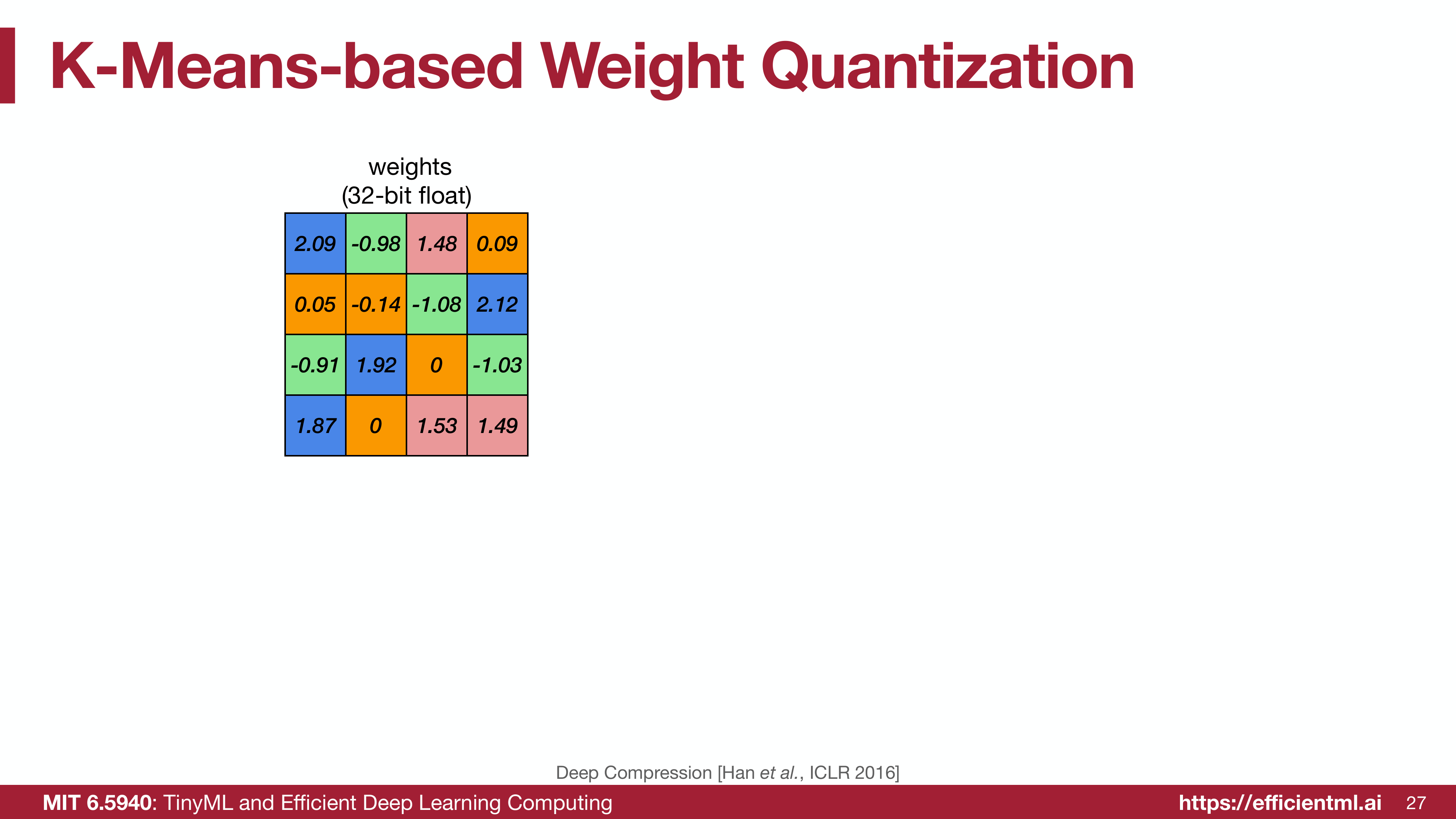Original weights before quantization

How K-Means Clustering Works for Weights

The process follows standard K-means clustering with a neural network twist.

Step 1: Initialize Cluster Centroids

Start by selecting k initial centroid values. Common initialization strategies include:

Random selection: Pick k random weights from the layer as initial centroids.

Linear initialization: Distribute centroids evenly across the weight range:

\[c_i = w_{\text{min}} + \frac{i}{k-1}(w_{\text{max}} - w_{\text{min}}), \quad i = 0, 1, ..., k-1\]

Density-based initialization: Place more centroids where weights are concentrated.

Step 2: Assign Weights to Nearest Centroid

For each weight $w_j$, find the closest centroid $c_i$ using Euclidean distance:

\[\text{cluster}(w_j) = \arg\min_i |w_j - c_i|\]

This assignment creates k groups of weights, each represented by a cluster index.

Step 3: Update Centroids

Recalculate each centroid as the mean of all weights assigned to it:

\[c_i = \frac{1}{|S_i|} \sum_{w_j \in S_i} w_j\]

where $S_i$ is the set of weights belonging to cluster $i$.

Step 4: Iterate Until Convergence

Repeat steps 2-3 until centroids stabilize or a maximum iteration count is reached. Typically, convergence occurs within 10-20 iterations for neural network weights.

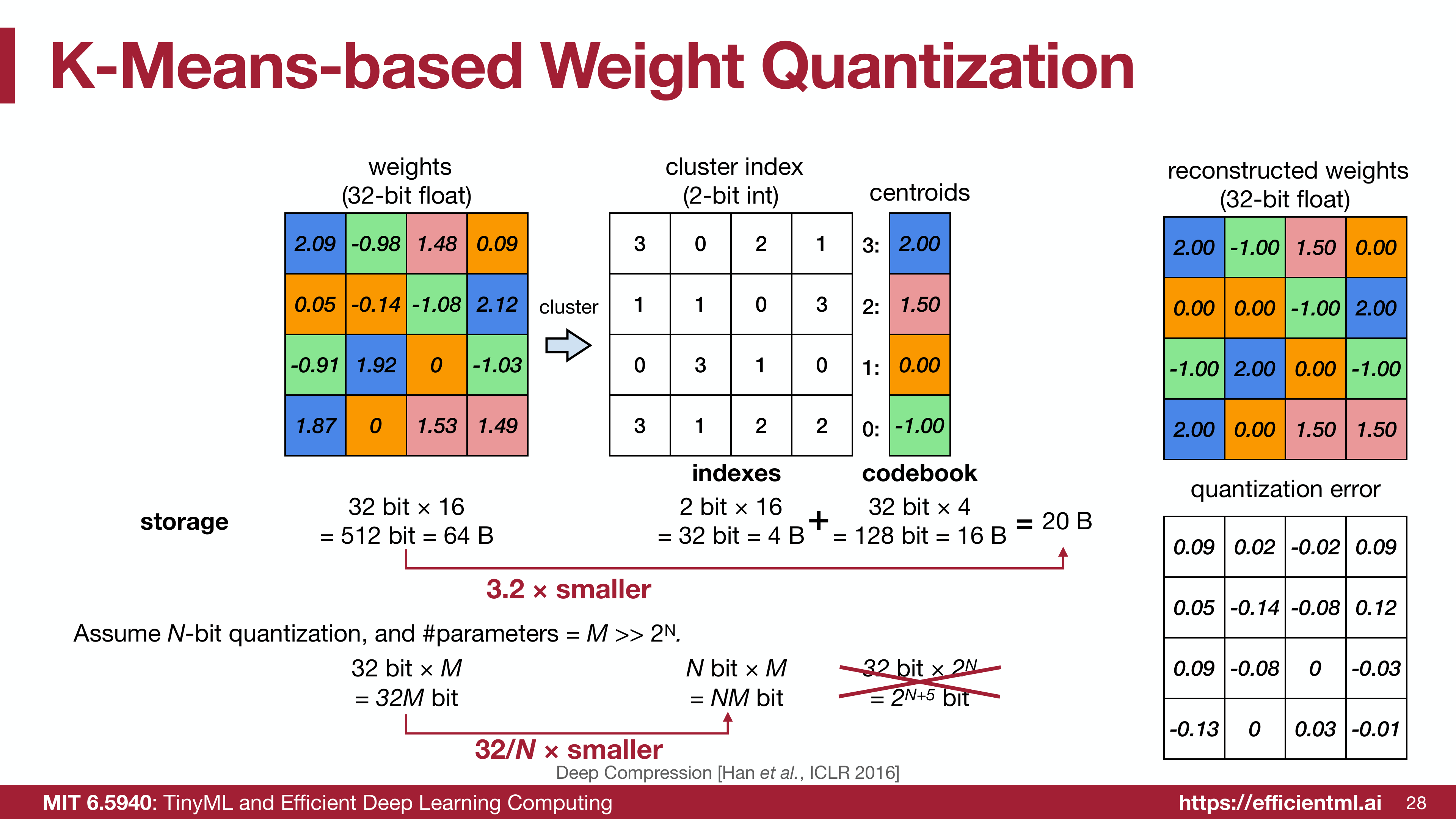K-means quantization showing indices, centroids, and reconstructed weights

Compression Ratio Analysis

Let’s analyze the storage savings mathematically. For a layer with M parameters using N-bit quantization:

Original storage: $32M$ bits (assuming FP32 weights)

Quantized storage:

• Indices: $NM$ bits (N bits per weight)
• Codebook: $32 \times 2^N$ bits (32-bit float for each of $2^N$ centroids)
• Total: $NM + 2^{N+5}$ bits

Compression ratio:

\[\text{Compression} = \frac{32M}{NM + 2^{N+5}} \approx \frac{32}{N} \quad \text{(when } M \gg 2^N\text{)}\]

For large layers where the codebook overhead becomes negligible:

• 2-bit quantization: 16× compression
• 3-bit quantization: 10.7× compression
• 4-bit quantization: 8× compression
• 8-bit quantization: 4× compression

The approximation $32/N$ holds because the codebook size $2^{N+5}$ becomes insignificant compared to $NM$ for typical neural network layers with millions of parameters.

Quantization Error and Reconstruction

After quantization, each weight is replaced by its cluster centroid. This introduces quantization error:

\[\epsilon_j = w_j - c_{\text{cluster}(w_j)}\]

The reconstruction process is straightforward—each quantized weight index maps to its centroid value via a lookup table (codebook):

\[\tilde{w}_j = c_{\text{cluster}(w_j)}\]

The total quantization error for a layer is:

\[E = \sum_{j=1}^M \epsilon_j^2 = \sum_{j=1}^M (w_j - \tilde{w}_j)^2\]

K-means clustering minimizes this squared error, making it optimal in the mean-squared-error sense.

Fine-Tuning Quantized Weights

Initial quantization typically degrades accuracy because we’re replacing precise weights with coarser cluster representatives. The solution? Fine-tune the centroids using backpropagation while keeping cluster assignments fixed.

Gradient Computation

During forward pass, weights are reconstructed using the codebook:

\[\tilde{w}_j = c_{\text{cluster}(w_j)}\]

During backward pass, we compute gradients with respect to the loss function $L$:

\[\frac{\partial L}{\partial c_i} = \sum_{j: \text{cluster}(w_j) = i} \frac{\partial L}{\partial \tilde{w}_j}\]

This means the gradient for each centroid is the sum of gradients from all weights in that cluster.

Gradient aggregation for centroid updates during fine-tuning

Centroid Update Rule

Update centroids using standard gradient descent:

\[c_i \leftarrow c_i - \eta \frac{\partial L}{\partial c_i}\]

where $\eta$ is the learning rate. This process adapts the centroids to minimize the loss function while maintaining the quantization structure.

Important Considerations

Fixed cluster assignments: During fine-tuning, weight-to-cluster assignments remain fixed. Only centroid values update. This prevents cluster instability during training.

Learning rate scheduling: Use a smaller learning rate than initial training—typically 1/10th or less—to avoid disrupting the learned representations.

Number of epochs: Fine-tuning usually requires far fewer epochs than full training, often 10-20% of the original training duration.

Compression Results on Real Networks

The Deep Compression paper demonstrated impressive results on ImageNet classification:

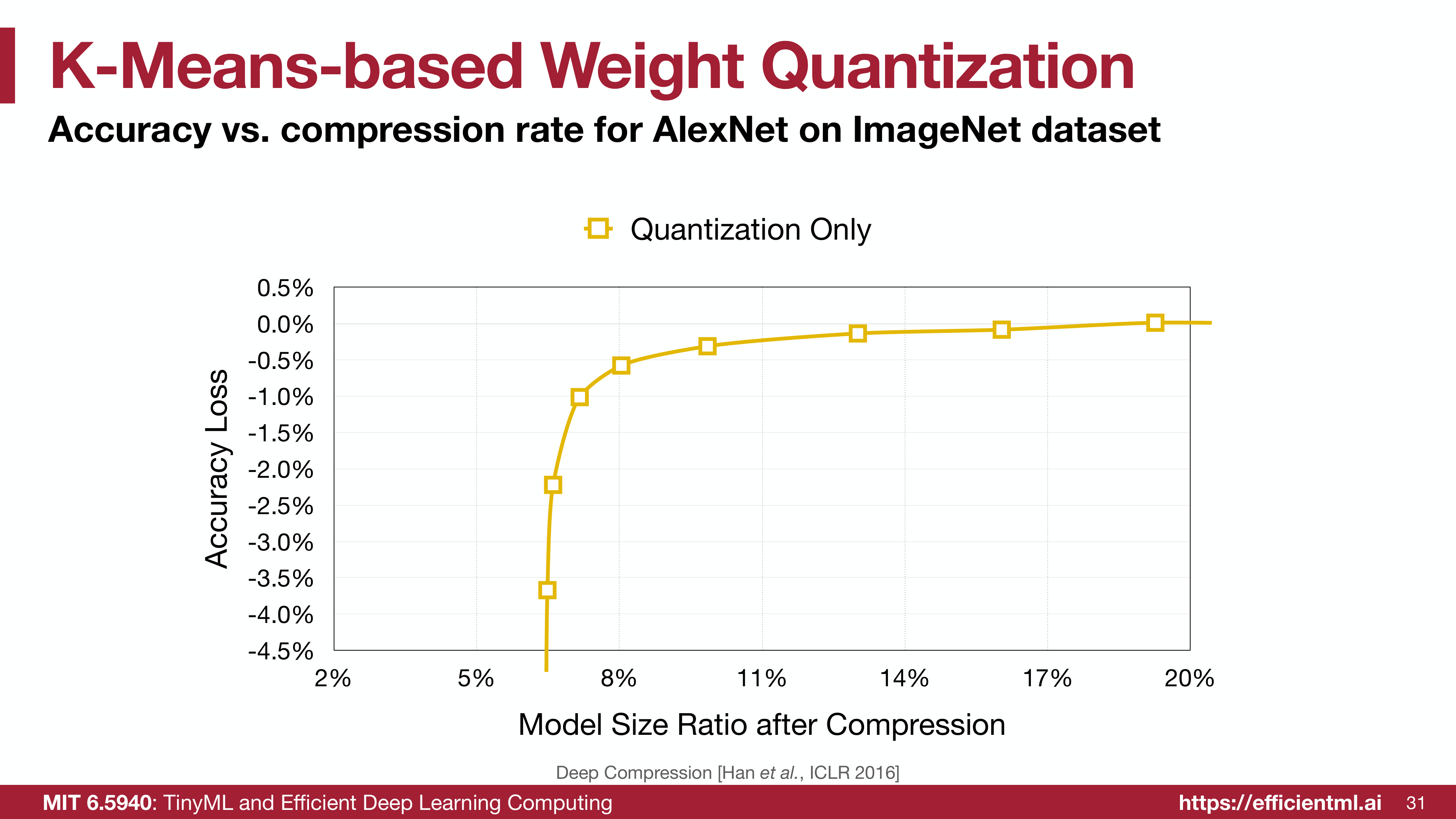
Quantization achieves significant compression with minimal accuracy loss

AlexNet (240 MB → 6.9 MB):

• 35× compression with quantization alone
• Maintains 80.27% top-1 accuracy (same as baseline)
• When combined with pruning: 49× compression

VGGNet (550 MB → 11.3 MB):

• 49× compression
• Actually improves accuracy from 88.68% to 89.09%
• The quantization acts as implicit regularization

ResNet-18 (44.6 MB → 4.0 MB):

• 11× compression
• Negligible accuracy degradation (89.24% → 89.28%)

Weight Distribution Evolution

An fascinating observation: quantization changes weight distributions in predictable ways.

Continuous weight distribution before quantization

Before quantization: Weights follow a relatively smooth, continuous distribution, often approximating a Gaussian centered near zero.

After initial quantization: The distribution becomes discretized with sharp peaks at centroid values. Weights between centroids disappear, creating gaps.

After fine-tuning: The distribution adjusts further, with centroids shifting to positions that minimize loss. Clusters may become unbalanced, with some centroids capturing many weights while others capture few.

This evolution reveals how the network adapts to the quantization constraint, finding configurations that maintain functionality despite reduced precision.

The Deep Compression Pipeline

K-means quantization shines when combined with other compression techniques in the Deep Compression pipeline:

Three-Stage Compression

Stage 1 - Pruning: Remove unimportant connections (typically 90% of weights)

• Result: 9-13× compression

Stage 2 - Quantization: Apply K-means clustering to remaining weights

• Result: 27-31× cumulative compression

Stage 3 - Huffman Coding: Variable-length encoding based on frequency

• Result: 35-49× final compression
• Same accuracy as original model

The synergy between these techniques is remarkable. Pruning removes the least important weights, making the remaining weights easier to quantize. Huffman coding then exploits the non-uniform distribution of cluster indices to squeeze out additional bits.

Deployment Considerations

Storage Format

The quantized model stores:

• Weight indices: Packed efficiently (e.g., 4 weights per byte for 2-bit quantization)
• Codebook: Array of floating-point centroids
• Cluster assignments: Metadata mapping indices to codebook positions

Runtime Inference

During inference, K-means quantization requires weight decompression:

1. Read quantized index for each weight
2. Look up corresponding centroid in codebook
3. Use reconstructed floating-point weight in computation

Critical insight: All computation remains in floating-point. K-means quantization only saves storage—it doesn’t accelerate computation or reduce memory bandwidth during inference.

This contrasts with linear quantization (covered in Part 3), which enables integer arithmetic throughout the entire inference pipeline.

Memory Access Patterns

Modern GPUs and CPUs cache decompressed weights, amortizing the lookup cost:

• First access: Read index, perform codebook lookup
• Subsequent accesses: Use cached floating-point value
• Memory bandwidth: Reduced by compression ratio for initial load

Practical Implementation Tips

Choosing the Number of Clusters

Start conservative: Begin with 256 clusters (8-bit indices) and gradually reduce:

\[k \in \{256, 128, 64, 32, 16\}\]

Monitor accuracy degradation at each step. Different layers may tolerate different compression levels.

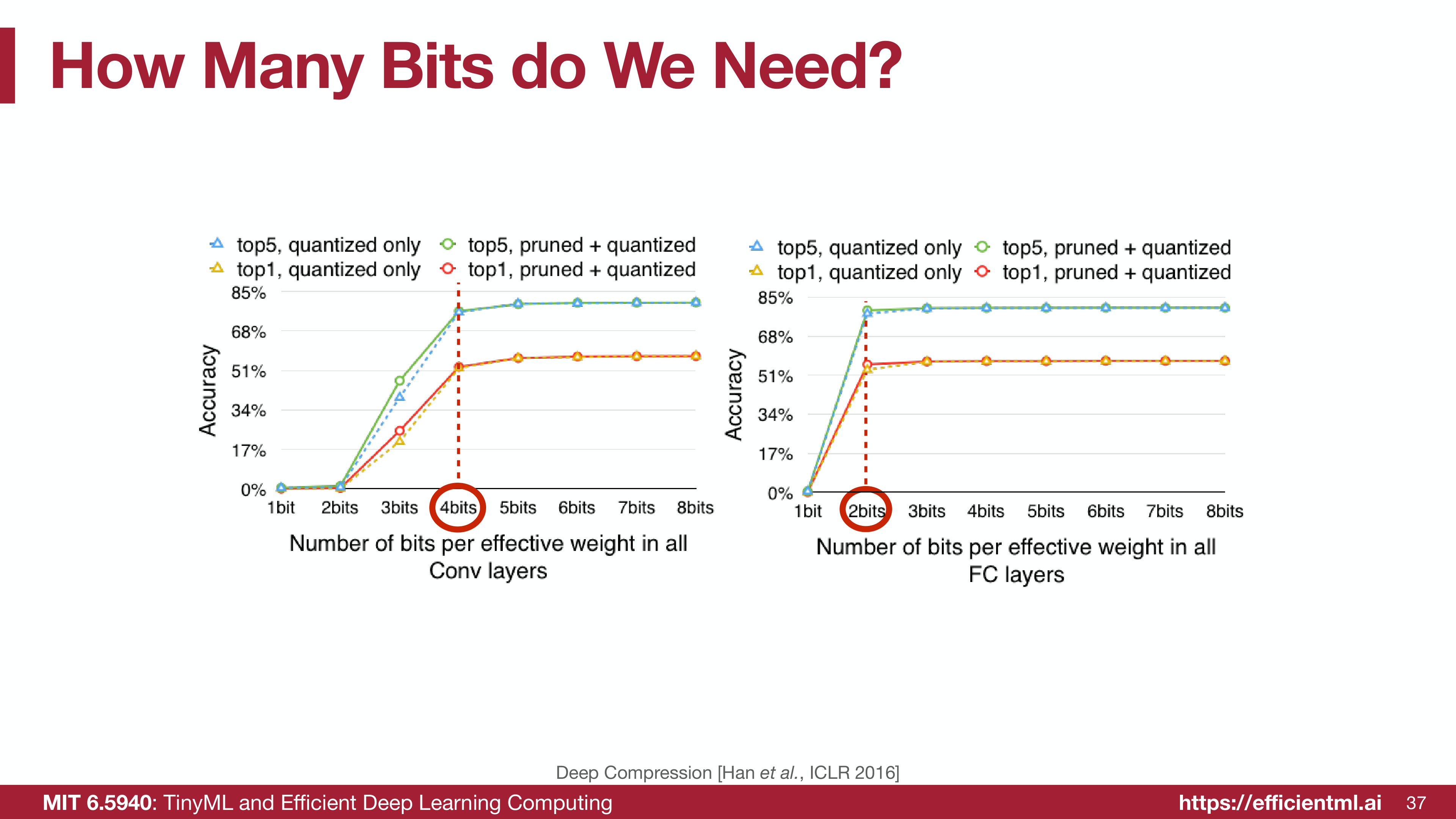
Layer-wise adaptation: Convolutional layers often tolerate more aggressive quantization (4-bit) than fully-connected layers (6-8 bit). The first and last layers are typically most sensitive.

Quantization granularity: Apply K-means per layer or per channel. Per-channel quantization typically preserves accuracy better but increases codebook overhead.

Initialization Strategies

Hybrid initialization: Combine linear spacing with density awareness:

1. Compute weight histogram
2. Place more centroids in dense regions
3. Ensure coverage of outliers

This balances between covering the full range and accurately representing common values.

Fine-Tuning Best Practices

Gradual quantization: Don’t quantize all layers simultaneously. Instead:

1. Quantize less sensitive layers first
2. Fine-tune until accuracy recovers
3. Gradually quantize more layers

Layer freezing: During fine-tuning, consider freezing already-quantized layers to prevent quality degradation.

Validation monitoring: Track validation accuracy closely. Stop fine-tuning if accuracy stops improving to avoid overfitting.

Limitations and Trade-offs

Computational Overhead

No speedup: K-means quantization doesn’t accelerate inference since all operations remain floating-point. It only saves storage and model loading time.

Lookup latency: Codebook lookups introduce overhead, especially for small batch sizes where caching is less effective.

Accuracy Constraints

Extreme quantization challenges: Below 4 bits, maintaining accuracy becomes difficult without sophisticated techniques like mixed-precision or layer-specific bit widths.

Task dependency: Classification tasks tolerate quantization better than tasks requiring fine-grained predictions (e.g., depth estimation, semantic segmentation).

Hardware Compatibility

Limited hardware support: Unlike linear quantization, K-means quantization lacks specialized hardware support. Most accelerators target integer arithmetic, not codebook lookups.

When to Use K-Means Quantization

K-means quantization excels in specific scenarios:

Model distribution: When model size dominates deployment concerns (e.g., downloading models to mobile devices)

Storage-constrained systems: Embedded devices with limited flash memory but adequate compute capability

Model versioning: Maintaining multiple model versions where storage costs accumulate

Combined with pruning: Achieving maximum compression when combined with structured or unstructured pruning

However, for inference acceleration, linear quantization (Part 3) typically provides better results due to hardware support for integer operations.

Key Takeaways

• K-means treats quantization as clustering: Groups similar weights together with shared centroids
• Storage compression: Achieves $32/N$× compression for N-bit quantization
• Fine-tuning essential: Centroid adjustment via backpropagation recovers most accuracy loss
• Floating-point computation: All inference operations remain in floating-point—only storage is compressed
• Deep Compression synergy: Combines with pruning and Huffman coding for 35-49× compression
• Layer sensitivity varies: Different layers tolerate different quantization levels
• No inference speedup: Unlike linear quantization, K-means doesn’t accelerate computation

Looking Forward

K-means quantization demonstrates that neural networks can tolerate substantial precision reduction in storage without accuracy loss. However, its reliance on floating-point computation during inference limits its efficiency gains.

In Part 3, we’ll explore linear quantization, which takes the next step: enabling integer arithmetic throughout the entire inference pipeline. By carefully mapping floating-point values to integers with affine transformations, linear quantization achieves both storage compression and computational acceleration—making it the dominant approach in production deployment.

---

Series Navigation:

• Part 1: Understanding Numeric Data Types
• Part 2: K-Means Based Weight Quantization (Current)
• Part 3: Linear Quantization Methods
• Part 4: Quantized Neural Network Operations
• Part 5: Post-Training Quantization Techniques
• Part 6: Quantization-Aware Training
• Part 7: Binary and Ternary Quantization
• Part 8: Mixed-Precision Quantization

References:

• MIT 6.5940: TinyML and Efficient Deep Learning Computing - EfficientML.ai Lecture 05: Quantization Part I (Fall 2024)
• Deep Compression: Compressing Deep Neural Networks with Pruning, Trained Quantization and Huffman Coding - Song Han et al., ICLR 2016
• SqueezeNet: AlexNet-level accuracy with 50x fewer parameters and <0.5MB model size - Iandola et al., 2016
• Neural Network Distiller: Quantization Documentation