Quantization Part 6: Quantization-Aware Training
Post-training quantization (Part 5) works remarkably well for INT8 deployment of large models, but it struggles when we push to 4-bit precision or work with smaller networks where representational capacity is limited. The solution? Train the neural network with quantization in mind from the start—or fine-tune it to adapt to quantization constraints. This is quantization-aware training (QAT), and it recovers most accuracy loss from aggressive quantization by teaching the model to be “quantization-friendly.”
The Core Insight
The fundamental idea behind QAT is elegant: if we want a model to perform well when quantized, we should simulate quantization during training so the model learns weights and activations that tolerate discretization.
Key principle: Maintain full-precision weights during training for gradient accumulation, but use quantized values in the forward pass to simulate deployment conditions.
This creates a feedback loop where the model learns to work around quantization constraints rather than fighting them.
Fake Quantization: Simulating Integer Inference
During QAT, we don’t actually use integer arithmetic—that would make training impractical. Instead, we use “fake quantization” (also called “simulated quantization”) that mimics the quantization effect while keeping everything in floating-point.
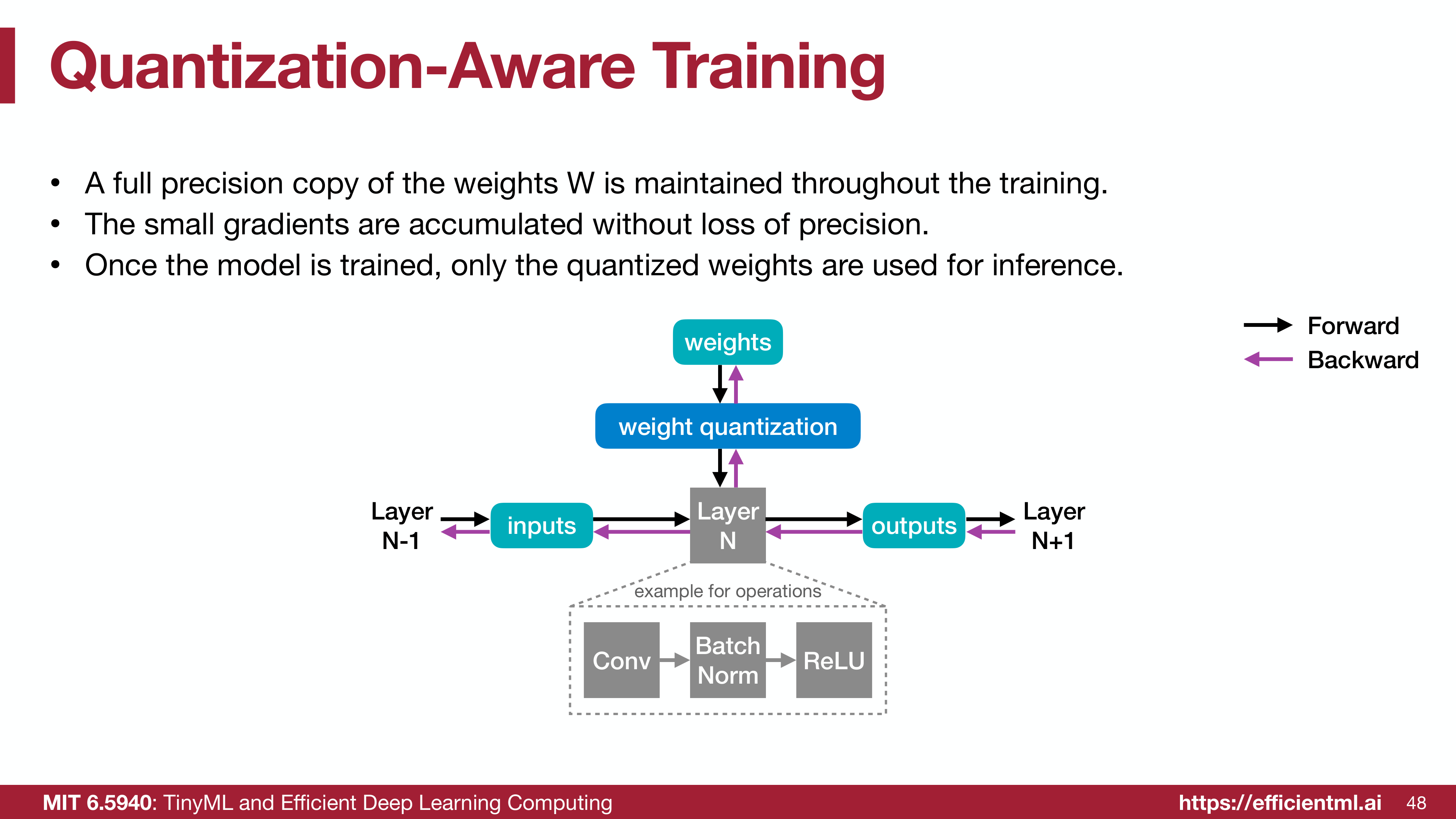 QAT maintains full-precision weights but simulates quantization in forward pass
The Fake Quantization Node
For weights, fake quantization applies the quantize-dequantize cycle:
\[W \rightarrow S_W \cdot q_W = Q(W)\]where:
\[q_W = \text{clip}\left(\text{round}\left(\frac{W}{S_W} + Z_W\right), q_{\min}, q_{\max}\right)\] \[Q(W) = S_W \cdot (q_W - Z_W)\]Critical observation: $Q(W)$ is in floating-point format but only takes discrete values that correspond to integer grid points. The neural network sees these quantized values during forward propagation, forcing it to learn representations that work despite the discretization.
Similarly, for activations:
\[Y \rightarrow S_Y \cdot (q_Y - Z_Y) = Q(Y)\]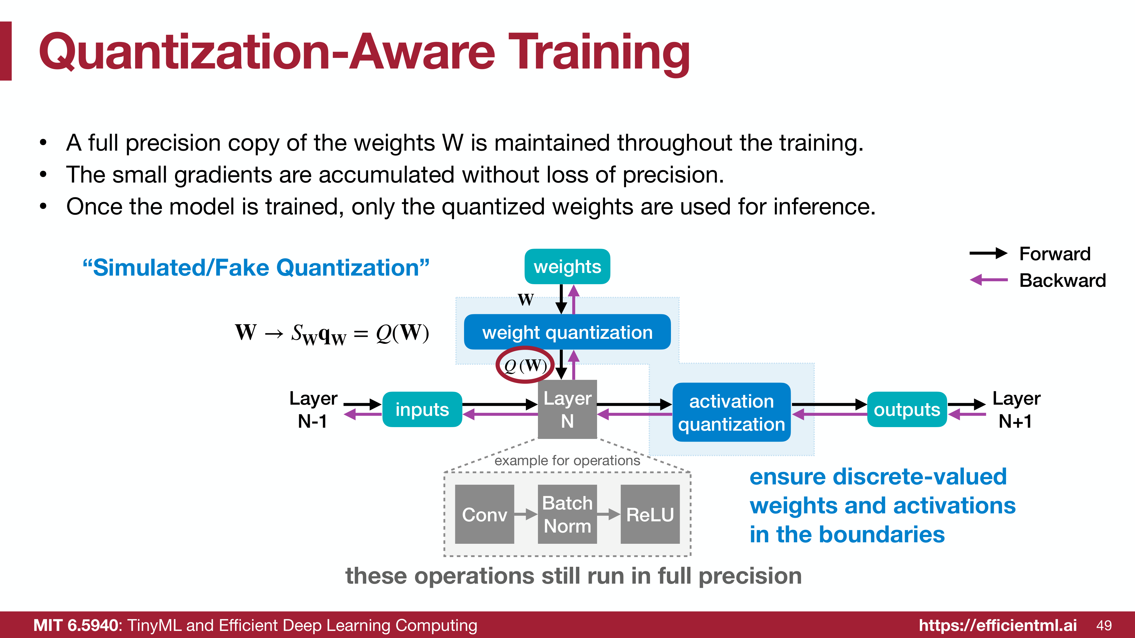 Fake quantization ensures discrete-valued weights and activations in forward pass while maintaining full-precision for gradient accumulation
Why “Fake”?
The term “fake” emphasizes that:
- Storage: Full-precision weights $W$ are maintained and updated
- Computation: Operations remain in floating-point (no integer arithmetic)
- Simulation: Only the discrete value constraint is enforced
- Deployment: After training, only quantized weights $q_W$ are stored and used
This distinction is crucial—QAT prepares the model for integer inference without actually performing integer operations during training.
The Gradient Problem
Quantization introduces a fundamental challenge for backpropagation: the quantization function $Q(W)$ involves rounding, which is non-differentiable.
\[\frac{\partial Q(W)}{\partial W} = \frac{\partial \text{round}(W/S_W + Z_W)}{\partial W} = 0 \text{ (almost everywhere)}\]If we naively compute gradients, we get:
\[\frac{\partial L}{\partial W} = \frac{\partial L}{\partial Q(W)} \cdot \frac{\partial Q(W)}{\partial W} = \frac{\partial L}{\partial Q(W)} \cdot 0 = 0\]Zero gradients mean no learning—the model would never improve!
Straight-Through Estimator (STE)
The solution is the Straight-Through Estimator, a simple but powerful trick: pretend the quantization function is the identity function when computing gradients.
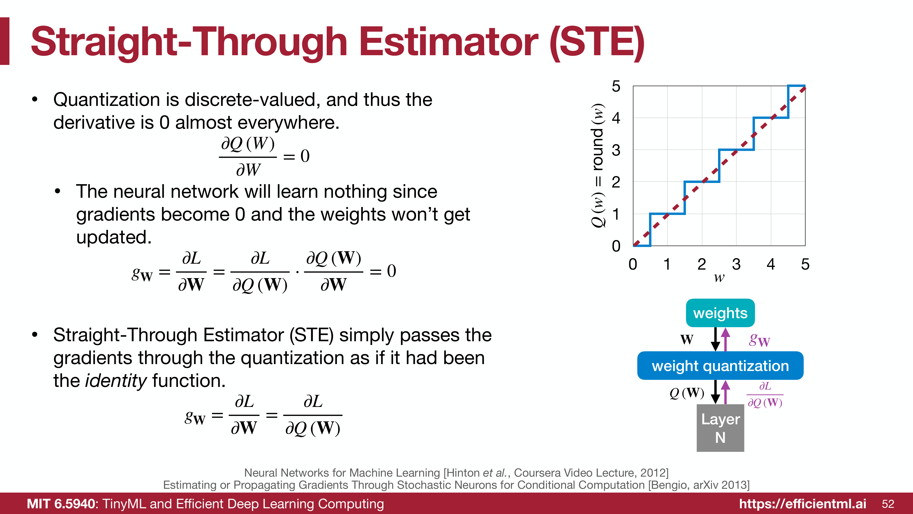 STE passes gradients through quantization as if it were identity
This gives us:
\[g_W = \frac{\partial L}{\partial W} = \frac{\partial L}{\partial Q(W)} \cdot \underbrace{\frac{\partial Q(W)}{\partial W}}_{\approx 1} = \frac{\partial L}{\partial Q(W)}\]Forward pass: Use quantized values $Q(W)$
Backward pass: Gradient flows through as if quantization didn’t exist
Intuition: The gradient tells us “how to change $W$ to reduce loss if $W$ could be anything.” Since $W$ can only take discrete values after quantization, this isn’t perfect—but empirically, it works remarkably well.
Why Does STE Work?
Several factors contribute to STE’s effectiveness:
1. Stochastic gradient descent naturally adds noise: Small gradient errors from STE are similar to the noise inherent in SGD with mini-batches.
2. Quantization is locally smooth: For weights far from quantization boundaries, small changes in $W$ don’t change $Q(W)$, making the identity approximation reasonable.
3. Training adapts: The model learns to position weights away from quantization boundaries where STE is least accurate, making the approximation self-improving.
4. Full-precision accumulation: Maintaining $W$ in full precision allows small gradients to accumulate over many steps, eventually moving weights across quantization boundaries.
QAT Training Pipeline
Complete Training Flow
The full QAT pipeline maintains dual representations:
Complete QAT pipeline showing fake quantization for both weights and activations
Full-precision shadow weights ($W$):
- Updated by gradients
- Accumulate small changes over many iterations
- Never used in forward pass
- Discarded after training
Quantized values ($Q(W)$, $Q(Y)$):
- Used in forward pass
- Simulate deployment conditions
- Discrete values only
- Converted to integers for deployment
Training Algorithm
1
2
3
4
5
6
7
8
9
10
11
12
13
14
15
16
17
18
19
20
21
22
23
24
25
26
# Pseudocode for QAT training loop

for epoch in epochs:
    for batch in dataloader:
        # Forward pass with fake quantization
        x = batch['input']

        # Quantize activations
        x_quantized = fake_quantize(x, S_x, Z_x)

        # Quantize weights
        W_quantized = fake_quantize(W, S_W, Z_W)

        # Forward pass with quantized values
        output = model_forward(x_quantized, W_quantized)

        loss = compute_loss(output, batch['target'])

        # Backward pass (STE gradients)
        loss.backward()  # Gradients computed w.r.t. full-precision W

        # Update full-precision weights
        optimizer.step(W)  # W updated, not W_quantized

        # Update quantization parameters (optional)
        update_scale_and_zeropoint(W, activations)
Layer-by-Layer Integration
Each layer in the network incorporates fake quantization:
Convolutional layer:
1
2
3
4
5
6
7
8
9
10
11
12
13
14
# Full-precision weights maintained
self.weight = nn.Parameter(torch.randn(out_ch, in_ch, k, k))

def forward(self, x):
    # Quantize input activations
    x_q = fake_quantize(x, self.S_x, self.Z_x)

    # Quantize weights
    w_q = fake_quantize(self.weight, self.S_W, self.Z_W)

    # Convolution with quantized values
    y = F.conv2d(x_q, w_q, bias=self.bias)

    return y
Activation functions:
1
2
3
4
5
6
7
8
def quantized_relu(x):
    # Apply ReLU
    y = F.relu(x)

    # Quantize output
    y_q = fake_quantize(y, S_y, Z_y)

    return y_q
QAT vs PTQ: Accuracy Comparison
The accuracy improvement from QAT over PTQ is substantial, especially for aggressive quantization:
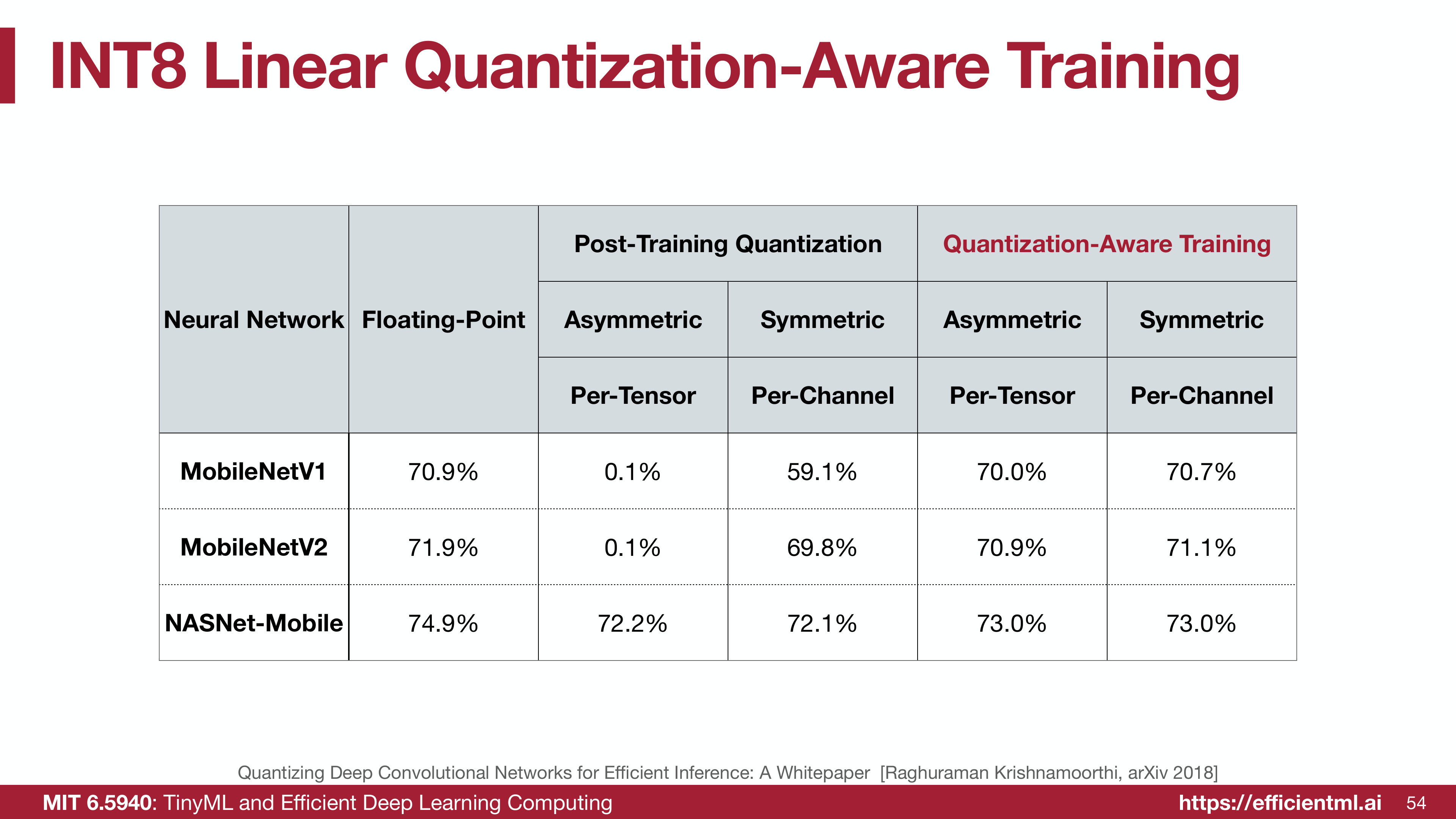 QAT significantly improves accuracy for small models
INT8 Results
| Network | FP32 | PTQ Asymmetric | PTQ Symmetric | QAT Asymmetric | QAT Symmetric |
|---|---|---|---|---|---|
| MobileNetV1 | 70.9% | 0.1% | 59.1% | 70.0% | 70.7% |
| MobileNetV2 | 71.9% | 0.1% | 69.8% | 70.9% | 71.1% |
| NASNet-Mobile | 74.9% | - | 72.2% | 73.0% | 73.0% |
Key observations:
MobileNetV1: PTQ symmetric quantization catastrophically fails (11.8% accuracy loss), but QAT recovers to only 0.2% loss—a 11.6 percentage point improvement!
MobileNetV2: PTQ loses 2.1%, QAT loses only 0.8%—a 1.3 pp improvement.
General trend: Smaller models benefit more from QAT because their limited capacity makes each bit of precision more valuable.
INT4 and Lower
For ultra-low precision, QAT becomes essential:
| Precision | PTQ Accuracy Loss | QAT Accuracy Loss |
|---|---|---|
| INT8 | 0.5-2% | 0.1-0.5% |
| INT6 | 1-3% | 0.3-1% |
| INT4 | 3-6% | 1-2% |
| INT2 | 10-20% | 3-8% |
QAT recovers 50-75% of the quantization error compared to PTQ.
Fine-Tuning Strategies
Starting from a pretrained FP32 model and fine-tuning with QAT typically works better than training from scratch with quantization.
Recommended Fine-Tuning Recipe
1. Learning rate: Use 1/10th to 1/100th of initial training rate
1
2
base_lr = 0.1  # Original training
qat_lr = 0.01  # QAT fine-tuning
2. Epochs: 10-20% of original training duration usually sufficient
1
2
original_epochs = 100
qat_epochs = 10-20
3. Batch normalization: Freeze BN statistics or use small momentum
1
2
3
4
5
for module in model.modules():
    if isinstance(module, nn.BatchNorm2d):
        module.momentum = 0.01  # Reduce from default 0.1
        # Or freeze completely:
        # module.eval()
4. Gradual quantization: Start with higher precision, gradually reduce
1
2
3
# Epoch 0-5: INT8
# Epoch 6-10: INT6
# Epoch 11-15: INT4
5. Layer freezing: Progressively freeze layers from input to output
1
2
3
4
# Freeze early layers first (they're more sensitive)
for layer_idx in range(num_layers):
    if epoch > layer_idx * freeze_schedule:
        freeze_layer(model.layers[layer_idx])
Learning Rate Scheduling
Cosine annealing with warm restart works well:
\[\eta_t = \eta_{\min} + \frac{1}{2}(\eta_{\max} - \eta_{\min})\left(1 + \cos\left(\frac{T_{\text{cur}}}{T_{\max}}\pi\right)\right)\]This allows the model to escape local minima caused by quantization constraints.
Advanced QAT Techniques
Learnable Quantization Parameters
Instead of fixing scale factors, make them learnable:
\[S_W = \text{learnable\_parameter}()\]This allows the network to optimize the quantization grid itself:
1
2
3
4
5
self.scale_W = nn.Parameter(torch.tensor(1.0))
self.zero_point_W = nn.Parameter(torch.tensor(0.0))

def quantize_weights(self):
    return fake_quantize(self.weight, self.scale_W, self.zero_point_W)
Benefit: Automatically finds optimal quantization ranges per layer.
Caution: Can lead to unstable training if not carefully regularized.
Per-Channel QAT
Extend QAT to per-channel quantization for better accuracy:
1
2
3
4
5
6
7
8
9
10
11
# Per-channel scale factors
self.scale_W = nn.Parameter(torch.ones(out_channels))

def quantize_weights(self):
    # Different scale per output channel
    w_q = []
    for i in range(self.out_channels):
        w_i = self.weight[i, :, :, :]
        w_i_q = fake_quantize(w_i, self.scale_W[i], self.zero_point_W[i])
        w_q.append(w_i_q)
    return torch.stack(w_q)
Mixed-Precision QAT
Train with different bit-widths for different layers:
1
2
3
4
5
6
7
# Sensitive layers: higher precision
self.layer1.set_precision(8)  # INT8
self.layer2.set_precision(8)

# Robust layers: lower precision
self.layer10.set_precision(4)  # INT4
self.layer11.set_precision(4)
This will be explored in depth in Part 8.
Deployment Workflow
From QAT Model to Production
Step 1: Train with QAT
1
model_qat = train_with_quantization_aware()
Step 2: Convert to integer-only
1
2
3
4
5
6
7
8
9
# Extract quantized weights
W_int8 = quantize_to_int8(model_qat.weight)

# Extract scale factors and zero points
scales = model_qat.scales
zero_points = model_qat.zero_points

# Save integer model
save_model(W_int8, scales, zero_points)
Step 3: Deploy with integer inference
1
2
3
4
5
6
7
8
9
# Load quantized model
W_int8, scales, zero_points = load_model()

# Integer-only inference
def inference(x_int8):
    # All operations in INT8
    y_int32 = matmul_int8(W_int8, x_int8)
    y_int8 = requantize(y_int32, scales)
    return y_int8
Verification
Always validate that integer inference matches QAT predictions:
1
2
3
4
5
6
7
8
# QAT model output
y_qat = model_qat(x)

# Integer model output
y_int = integer_inference(quantize(x))

# Should be very close
assert torch.allclose(y_qat, dequantize(y_int), atol=1e-3)
Common Pitfalls and Solutions
Pitfall 1: Training Instability
Symptom: Loss oscillates or diverges during QAT fine-tuning.
Solution:
- Reduce learning rate further (try 1/100th or 1/1000th)
- Increase batch size for more stable gradients
- Use gradient clipping:
torch.nn.utils.clip_grad_norm_(model.parameters(), max_norm=1.0)
Pitfall 2: Batch Normalization Mismatch
Symptom: Training accuracy good but validation accuracy poor.
Solution:
- Freeze BN statistics:
model.eval()mode during QAT - Or use very small BN momentum (0.001-0.01)
- Recalibrate BN statistics after QAT using calibration set
Pitfall 3: Quantization Parameter Drift
Symptom: Scale factors become extremely large or small.
Solution:
- Clip scale factors to reasonable range [0.001, 100]
- Use regularization on scale parameters
- Initialize scales from PTQ calibration
Pitfall 4: First/Last Layer Sensitivity
Symptom: Quantizing first or last layer destroys accuracy.
Solution:
- Keep first/last layers in higher precision (FP16 or INT8)
- Apply QAT only to middle layers initially
- Use per-channel quantization for these sensitive layers
When to Use QAT vs PTQ
Use PTQ when:
- INT8 precision is sufficient
- Large models (>100M parameters)
- Limited training resources
- No access to training data
- Quick deployment needed
Use QAT when:
- <8-bit precision required (INT6, INT4, INT2)
- Small models (<50M parameters)
- Maximum accuracy critical
- Training infrastructure available
- Can afford fine-tuning time (days)
Hybrid Approach:
- Start with PTQ for quick baseline
- If accuracy insufficient, apply QAT
- Use QAT only for layers where PTQ fails
Key Takeaways
- QAT simulates quantization during training via fake quantization nodes
- Straight-Through Estimator enables gradient flow by treating quantization as identity in backward pass
- Dual representation: Full-precision weights updated by gradients, quantized values used in forward pass
- Substantial accuracy improvement: QAT recovers 50-75% of PTQ quantization error
- Essential for aggressive quantization: INT4 and below require QAT for acceptable accuracy
- Fine-tuning from FP32 works better than training from scratch with quantization
- Learning rate: Use 1/10th to 1/100th of original training rate
- Small models benefit most: MobileNets see 10+ percentage point improvements with QAT
- BN handling critical: Freeze or use small momentum to avoid train-test mismatch
Bridging to Extreme Quantization
Quantization-aware training enables aggressive compression to 4-bit and even lower. But can we push further? What happens at the extreme limit of 1-bit weights and activations?
Part 7 explores Binary and Ternary Quantization, where weights take only values {-1, +1} or {-1, 0, +1}. These extreme quantization schemes replace expensive multiplications with simple bit operations, enabling unprecedented speed and energy efficiency—but at the cost of significant accuracy trade-offs that require clever techniques to manage.
Series Navigation:
- Part 1: Understanding Numeric Data Types
- Part 2: K-Means Based Weight Quantization
- Part 3: Linear Quantization Methods
- Part 4: Quantized Neural Network Operations
- Part 5: Post-Training Quantization Techniques
- Part 6: Quantization-Aware Training (Current)
- Part 7: Binary and Ternary Quantization (Coming July 5, 2025)
- Part 8: Mixed-Precision Quantization (Coming July 10, 2025)
References:
- MIT 6.5940: TinyML and Efficient Deep Learning Computing - EfficientML.ai Lecture 06: Quantization Part II (Fall 2024)
- Quantizing Deep Convolutional Networks for Efficient Inference: A Whitepaper - Krishnamoorthi, arXiv 2018
- Estimating or Propagating Gradients Through Stochastic Neurons for Conditional Computation - Bengio et al., arXiv 2013
- Neural Networks for Machine Learning - Geoffrey Hinton, Coursera 2012
- Quantization and Training of Neural Networks for Efficient Integer-Arithmetic-Only Inference - Jacob et al., CVPR 2018