Quantization Part 4: Quantized Neural Network Operations
We’ve built the theoretical foundation for linear quantization in Part 3, establishing the affine mapping between integers and real numbers. Now comes the payoff: transforming neural network operations into pure integer arithmetic that runs blazingly fast on modern hardware. This final part reveals how matrix multiplications, convolutions, and activation functions operate entirely in the integer domain—unlocking the full potential of quantization.
The End-to-End Integer Challenge
The goal is elegant yet demanding: perform all neural network computations using only integer arithmetic, dequantizing to floating-point only at the final output layer. This maximizes hardware efficiency while maintaining accuracy comparable to floating-point inference.
The key insight? Every neural network operation can be expressed in terms of quantized values and precomputed scale factors, eliminating floating-point operations from the critical inference path.
Quantized Matrix Multiplication
Matrix multiplication forms the foundation of neural networks. Let’s derive its quantized form from first principles.
Starting Point
Consider the basic matrix multiplication:
\[Y = W \cdot X\]Substituting the linear quantization formula $r = S(q - Z)$:
\[S_Y(q_Y - Z_Y) = S_W(q_W - Z_W) \cdot S_X(q_X - Z_X)\]Expanding the right side:
\[S_Y(q_Y - Z_Y) = S_W S_X (q_W - Z_W)(q_X - Z_X)\] \[S_Y(q_Y - Z_Y) = S_W S_X (q_W q_X - Z_W q_X - Z_X q_W + Z_W Z_X)\]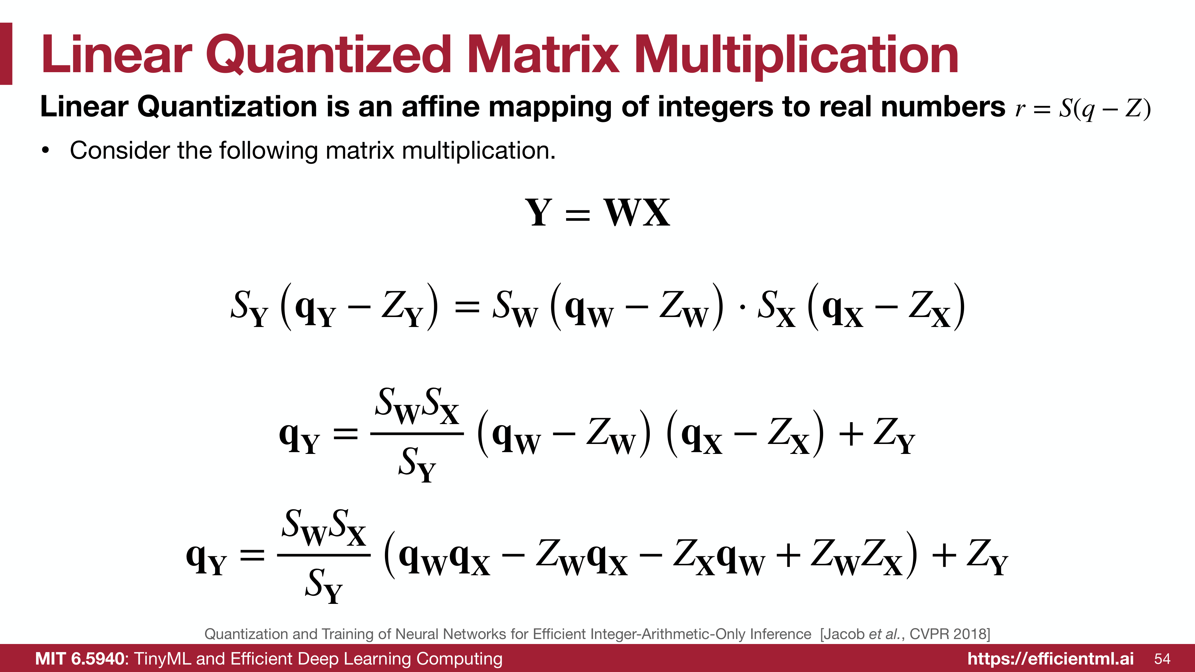 Deriving the quantized matrix multiplication formula
Solving for $q_Y$:
\[q_Y = \frac{S_W S_X}{S_Y}(q_W q_X - Z_W q_X - Z_X q_W + Z_W Z_X) + Z_Y\]Operation Breakdown
This equation reveals the complete integer-arithmetic pipeline:
Step 1: Compute $q_W q_X$ (N-bit × N-bit → 32-bit multiplication) Step 2: Subtract bias terms $Z_W q_X$ and $Z_X q_W$ (32-bit integer arithmetic) Step 3: Add $Z_W Z_X$ (precomputed 32-bit constant) Step 4: Multiply by combined scale $\frac{S_W S_X}{S_Y}$ (fixed-point multiplication) Step 5: Add zero point $Z_Y$ (N-bit integer addition)
Precomputation Opportunities
Notice that $Z_W$, $Z_X$, $Z_W Z_X$, and the combined scale are all known before inference. We can precompute:
\(C_1 = -Z_X q_W \quad \text{(precompute for each weight)}\) \(C_2 = Z_W Z_X \quad \text{(scalar constant)}\) \(M = \frac{S_W S_X}{S_Y} = 2^{-n} M_0, \quad M_0 \in [0.5, 1)\)
This reduces runtime computation significantly.
Simplification with Symmetric Weight Quantization
When weights use symmetric quantization ($Z_W = 0$), the formula simplifies dramatically:
\[q_Y = \frac{S_W S_X}{S_Y}(q_W q_X - Z_X q_W) + Z_Y\]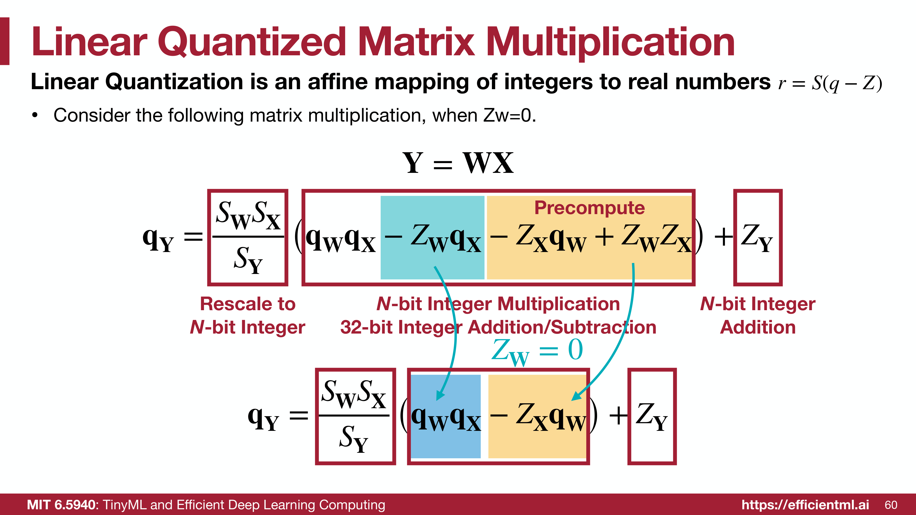 Computational graph with symmetric weight quantization
The $Z_W q_X$ term disappears, and $Z_W Z_X = 0$. We only need:
- Integer matrix multiplication $q_W q_X$
- Bias subtraction $Z_X q_W$ (precomputed per weight)
- Rescaling and zero-point addition
This is why most practical implementations use symmetric quantization for weights—the computational savings are substantial.
Quantized Fully-Connected Layer with Bias
Real neural network layers include bias terms. Let’s incorporate them:
\[Y = W \cdot X + b\]Substituting quantization:
\[S_Y(q_Y - Z_Y) = S_W(q_W - Z_W) \cdot S_X(q_X - Z_X) + S_b(q_b - Z_b)\]With $Z_W = 0$ (symmetric weights):
\[S_Y(q_Y - Z_Y) = S_W S_X(q_W q_X - Z_X q_W) + S_b(q_b - Z_b)\]Bias Quantization Strategy
A clever trick: quantize bias using the same scale as the weight-activation product:
\[S_b = S_W S_X, \quad Z_b = 0\]This allows direct addition of the bias to the accumulated products without additional rescaling:
\[S_Y(q_Y - Z_Y) = S_W S_X(q_W q_X - Z_X q_W + q_b)\]Solving for $q_Y$:
\[q_Y = \frac{S_W S_X}{S_Y}(q_W q_X + q_{\text{bias}}) + Z_Y\]where:
\[q_{\text{bias}} = q_b - Z_X q_W\]The term $q_{\text{bias}}$ is precomputed before inference, combining the original bias with the zero-point correction. This fused bias requires no additional arithmetic operations during inference.
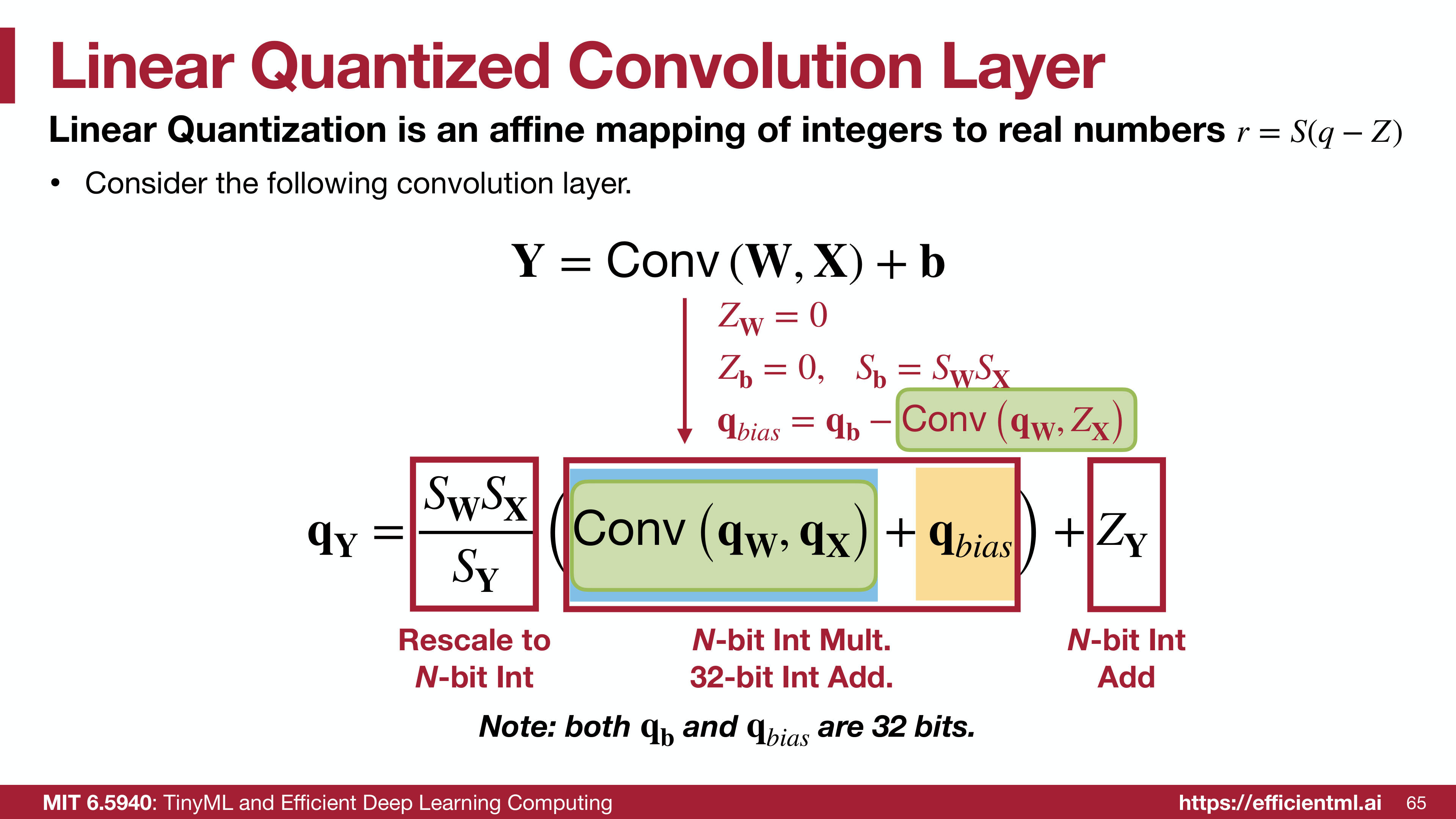 Complete quantized FC layer showing fused bias computation
Quantized Convolution Layer
Convolutions follow the same pattern as matrix multiplication but with spatial structure.
Derivation
Starting from:
\[Y = \text{Conv}(W, X) + b\]With symmetric weights ($Z_W = 0$) and fused bias scale ($S_b = S_W S_X$, $Z_b = 0$):
\[q_Y = \frac{S_W S_X}{S_Y}(\text{Conv}(q_W, q_X) + q_{\text{bias}}) + Z_Y\]where:
\[q_{\text{bias}} = q_b - \text{Conv}(q_W, Z_X)\]The key difference from FC layers: the zero-point correction $\text{Conv}(q_W, Z_X)$ now involves a convolution operation. However, since $Z_X$ is constant across all spatial positions, this simplifies to:
\[\text{Conv}(q_W, Z_X) = Z_X \sum_{k_h, k_w, c} q_W[c, k_h, k_w]\]This sum can be precomputed for each output channel, making it a simple per-channel scalar.
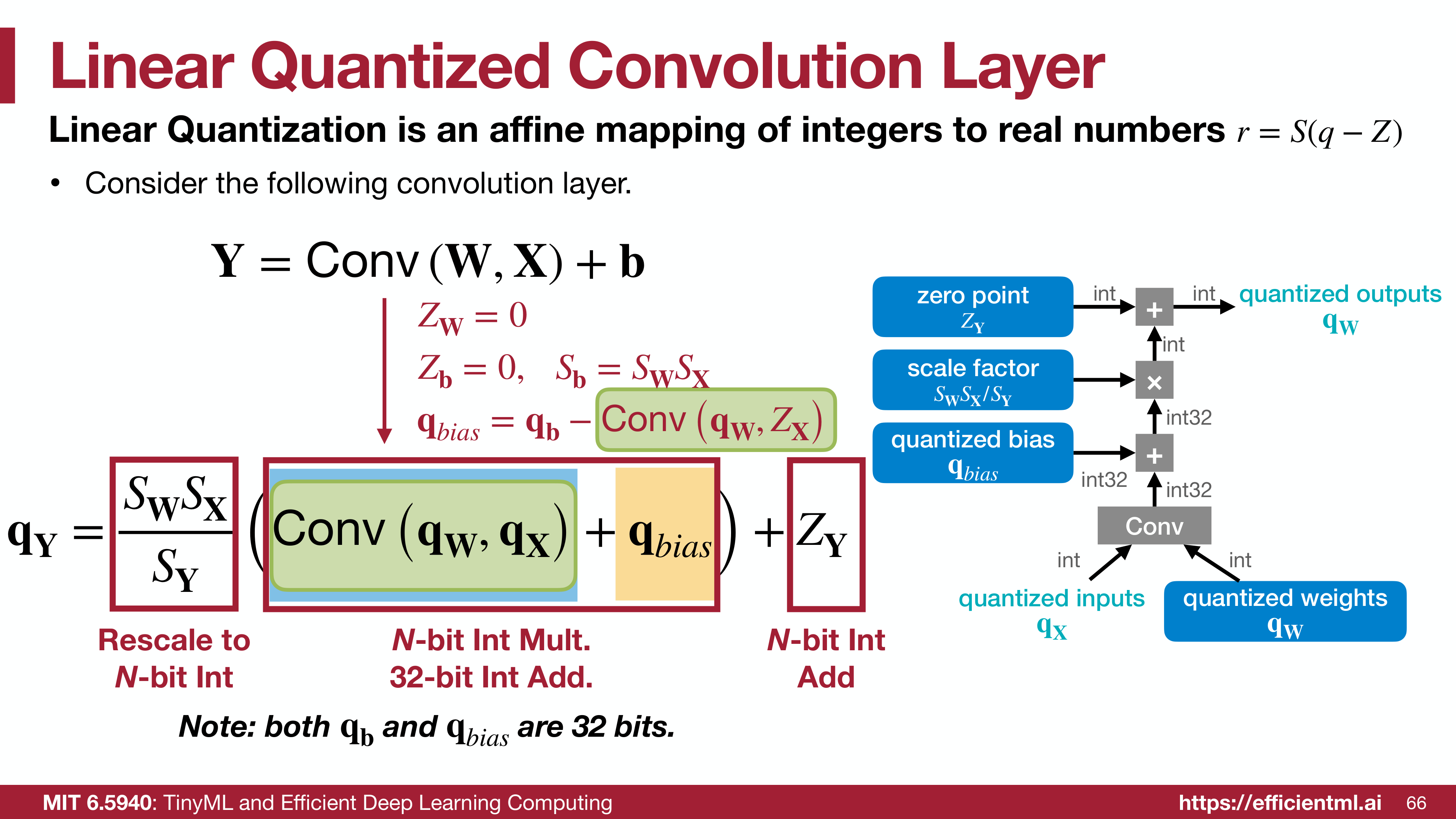 Quantized convolution pipeline with integer operations
Computational Flow
Let’s trace data through a quantized convolutional layer:
Inputs:
- Quantized activations $q_X$ (INT8)
- Quantized weights $q_W$ (INT8)
- Precomputed fused bias $q_{\text{bias}}$ (INT32)
- Scale factor $M = S_W S_X / S_Y$ (fixed-point)
- Zero point $Z_Y$ (INT8)
Computation Pipeline:
- Integer convolution:
- Compute $\text{Conv}(q_W, q_X)$ using INT8 × INT8 → INT32 multiply-accumulate
- Hardware accelerators (e.g., VNNI, DP4A) perform this extremely efficiently
- Bias addition:
- Add precomputed $q_{\text{bias}}$ (INT32 + INT32 → INT32)
- No additional memory access needed—bias is fused
- Rescaling:
- Multiply by fixed-point scale $M_0$ (INT32 × FP32 → INT32)
- Right-shift by $n$ bits (INT32 » n → INT32)
- This is the only “floating-point” operation, but modern hardware implements it in fixed-point
- Zero-point addition:
- Add $Z_Y$ (INT32 + INT8 → INT8)
- Clip to [-128, 127] to ensure valid INT8 range
- Output: Quantized activations $q_Y$ (INT8), ready for next layer
Efficient Rescaling Implementation
The rescaling step $\frac{S_W S_X}{S_Y}$ deserves special attention since it’s the only place floating-point appears.
Fixed-Point Representation
Express the combined scale as:
\[\frac{S_W S_X}{S_Y} = 2^{-n} \cdot M_0\]where $M_0 \in [0.5, 1)$ and $n$ is an integer shift amount.
In code:
1
2
3
4
5
6
7
8
9
10
11
def quantize_scale(scale):
    """Convert scale to fixed-point (shift, multiplier)."""
    # Find shift amount
    n = 0
    while scale < 0.5 and n < 31:
        scale *= 2
        n += 1

    # M0 is now in [0.5, 1), represent as INT32
    M0_int = int(scale * (2**31))
    return n, M0_int
Hardware Execution
Modern CPUs and accelerators implement this as:
1
2
3
4
5
6
7
8
9
10
11
// INT32 result from accumulation
int32_t acc = conv_result + bias;

// Fixed-point multiplication
int64_t scaled = (int64_t)acc * M0_int;

// Right shift and round
int32_t requantized = (int32_t)((scaled + (1 << (n + 30))) >> (n + 31));

// Add zero point and clip
int8_t output = clip(requantized + Z_Y, -128, 127);
The rounding constant $(1 « (n + 30))$ implements round-to-nearest instead of truncation.
Fused Operations
Modern quantized inference pipelines fuse multiple operations to minimize memory traffic.
Conv-BatchNorm-ReLU Fusion
Separate operations:
1
2
3
Y = Conv(W, X) + b
Y = BatchNorm(Y)
Y = ReLU(Y)
Fused implementation:
Fold BatchNorm parameters ($\gamma, \beta, \mu, \sigma$) into the convolution weights and bias:
\[W' = \frac{\gamma}{\sqrt{\sigma^2 + \epsilon}} \odot W\] \[b' = \frac{\gamma}{\sqrt{\sigma^2 + \epsilon}} \odot (b - \mu) + \beta\]Then quantize the fused $W’$ and $b’$. ReLU becomes a simple clipping operation:
\[q_Y = \max(q_Y, q_{\text{zero}})\]where $q_{\text{zero}}$ is the quantized representation of 0. For asymmetric quantization, $q_{\text{zero}} = Z_Y$.
Benefits
Memory traffic reduction: Single write to output instead of three separate writes Reduced quantization error: Only one quantize-dequantize cycle instead of three Improved throughput: Fewer memory bottlenecks
Handling Activation Functions
Different activation functions require different quantization strategies.
ReLU
The simplest case. For ReLU, we know $Y \geq 0$, so we can use asymmetric quantization with $r_{\min} = 0$:
\[q_Y = \max(q_Y, Z_Y) \quad \text{(where $Z_Y$ represents 0)}\]In integer arithmetic, this is a single comparison and conditional move—extremely efficient.
ReLU6
Clips to [0, 6], allowing optimization of the quantization range:
\[r_{\min} = 0, \quad r_{\max} = 6\] \[q_Y = \text{clip}(q_Y, Z_Y, q_{\text{max}})\]where $q_{\text{max}}$ is the quantized representation of 6.
Complex Activations (Sigmoid, Tanh, Swish)
Non-monotonic functions require lookup tables or piecewise linear approximation:
Lookup table approach:
- Precompute function values for all possible INT8 inputs
- Index into table during inference (256 entries for INT8)
Piecewise linear approximation:
- Approximate function as $y = ax + b$ over segments
- Store $(a, b)$ coefficients per segment
- Interpolate during inference
Performance Characteristics
Throughput Improvements
Quantized inference on modern hardware shows dramatic speedups:
NVIDIA T4 GPU (INT8 vs FP32):
- ResNet-50: 3.5× throughput increase
- BERT-Base: 2.8× throughput increase
Intel Cascade Lake CPU (INT8 VNNI):
- MobileNet-V2: 4.2× speedup
- ResNet-50: 3.1× speedup
ARM Cortex-A78 (INT8 NEON):
- MobileNet-V1: 5.3× speedup
- EfficientNet-B0: 4.7× speedup
Memory Bandwidth Reduction
INT8 models reduce memory traffic by 4× compared to FP32:
- Model size: 4× smaller
- Activation bandwidth: 4× less data transfer
- Cache utilization: More data fits in cache
This memory bandwidth reduction often matters more than raw compute speedup, especially for memory-bound models.
Energy Efficiency
As shown in Part 1, INT8 operations consume dramatically less energy:
- INT8 MAC: ~0.2 pJ
- FP32 MAC: ~3.7 pJ
- Improvement: 18.5× energy reduction per operation
For edge devices, this translates to longer battery life and reduced thermal constraints.
Accuracy Results
Real-world quantized models achieve excellent accuracy:
| Model | FP32 Top-1 | INT8 Top-1 | Degradation |
|---|---|---|---|
| ResNet-50 | 76.4% | 74.9% | -1.5% |
| Inception-V3 | 78.4% | 75.4% | -3.0% |
| MobileNet-V2 | 72.0% | 71.2% | -0.8% |
| EfficientNet-B0 | 77.1% | 76.8% | -0.3% |
With quantization-aware training, degradation typically drops below 0.5% for INT8 and 1-2% for INT4.
Implementation Best Practices
Layer-by-Layer Quantization
Strategy:
- Start with the first layer (often kept FP16/FP32)
- Quantize subsequent layers incrementally
- Validate accuracy after each layer
- Adjust bit-width if accuracy drops significantly
Sensitivity analysis: Plot accuracy vs quantization level per layer to identify sensitive layers.
Mixed-Precision Deployment
Not all layers need the same bit-width:
Common strategy:
- First and last layers: FP16 or INT8
- Intermediate convolutions: INT8
- Depthwise convolutions: INT8 or INT4
- Fully-connected layers: INT8
This balances accuracy and efficiency, keeping sensitive layers at higher precision while aggressively quantizing others.
Calibration Dataset Selection
Requirements:
- Representative of deployment distribution
- Covers diverse inputs (different classes, conditions)
- Size: 500-1000 samples typically sufficient
Avoid:
- Using training set (may overfit quantization to training data)
- Too small calibration sets (poor statistics)
- Biased samples (e.g., only easy examples)
Deployment Checklist
Before deploying quantized models:
Validation:
- Accuracy on full validation set within acceptable threshold
- Per-class accuracy checked for significant imbalances
- Edge cases tested (out-of-distribution inputs)
Performance:
- Measured actual inference latency on target hardware
- Memory bandwidth profiling completed
- Power consumption validated for mobile/edge devices
Correctness:
- Numerical equivalence tested (outputs match reference within tolerance)
- Bit-exact inference verified on target hardware
- Overflow/underflow handling validated
Key Takeaways
- Integer-only inference: All operations performed in INT8/INT4 arithmetic, dequantizing only at output
- Quantized matmul: $q_Y = \frac{S_W S_X}{S_Y}(q_W q_X - Z_W q_X - Z_X q_W + Z_W Z_X) + Z_Y$
- Symmetric weights ($Z_W = 0$) simplify computation dramatically
- Fused bias: $q_{\text{bias}} = q_b - Z_X q_W$ precomputed before inference
- Fixed-point rescaling: Combined scale represented as $2^{-n} M_0$ for efficient bit-shift
- Operation fusion: Conv-BN-ReLU fused into single operation reduces memory traffic
- Hardware acceleration: Modern processors include specialized INT8 instructions (VNNI, DP4A, Tensor Cores)
- 3-5× speedup: Typical throughput improvement over FP32 on modern hardware
- <1% accuracy loss: INT8 quantization with QAT maintains near-FP32 accuracy
The Complete Picture
We’ve now completed the quantization journey:
Part 1 established why lower precision matters—energy efficiency and computational throughput.
Part 2 introduced K-means quantization, demonstrating that neural networks tolerate clustering-based compression.
Part 3 derived linear quantization’s mathematical framework, enabling affine mapping between integers and reals.
Part 4 (this post) brought it all together, showing how to execute complete neural network inference using only integer arithmetic.
The result? Models that are 4× smaller, 3-5× faster, and consume 18× less energy per operation—with less than 1% accuracy degradation. This is quantization’s promise fulfilled: efficient deep learning that runs anywhere, from datacenter GPUs to mobile phones to tiny microcontrollers.
Next Steps in Your Quantization Journey
For practitioners:
- Start with post-training quantization (PTQ) for quick wins
- Profile your models to identify bottlenecks
- Use per-channel quantization for weights
- Experiment with mixed-precision for optimal accuracy-efficiency trade-off
For researchers:
- Explore sub-8-bit quantization (INT4, INT2)
- Investigate learned quantization parameters
- Develop hardware-aware quantization schemes
- Study theoretical bounds on quantization error
For hardware designers:
- Optimize INT8/INT4 MAC units
- Design efficient dequantization pipelines
- Support mixed-precision inference
- Minimize memory bandwidth requirements
The field continues to evolve, with emerging techniques like learned step size quantization, differentiable quantization, and binary neural networks pushing boundaries even further.
Series Navigation:
- Part 1: Understanding Numeric Data Types
- Part 2: K-Means Based Weight Quantization
- Part 3: Linear Quantization Methods
- Part 4: Quantized Neural Network Operations (Current)
- Part 5: Post-Training Quantization Techniques
- Part 6: Quantization-Aware Training
- Part 7: Binary and Ternary Quantization
- Part 8: Mixed-Precision Quantization
References:
- MIT 6.5940: TinyML and Efficient Deep Learning Computing - EfficientML.ai Lecture 05: Quantization Part I (Fall 2024)
- Quantization and Training of Neural Networks for Efficient Integer-Arithmetic-Only Inference - Jacob et al., CVPR 2018
- Integer Quantization for Deep Learning Inference: Principles and Empirical Evaluation - Wu et al., 2020
- A Survey of Quantization Methods for Efficient Neural Network Inference - Gholami et al., 2021
- TensorFlow Lite Quantization
- PyTorch Quantization Documentation