Quantization Part 5: Post-Training Quantization Techniques
Having mastered the fundamentals of linear quantization in Parts 1-4, we now face a practical challenge: how do we actually quantize an already-trained floating-point model without retraining? Post-training quantization (PTQ) answers this question, providing techniques to convert FP32 models to INT8 or lower precision with minimal accuracy loss—all without accessing the original training data or performing expensive fine-tuning.
The PTQ Challenge
Post-training quantization must determine optimal quantization parameters—scale factors and zero points—for every layer using only the trained model and a small calibration dataset. Three critical decisions dominate PTQ effectiveness:
- Quantization granularity: At what level do we apply quantization parameters?
- Dynamic range clipping: How do we handle outliers and determine min/max ranges?
- Rounding strategy: How do we optimally round weights to discrete values?
Each decision significantly impacts the accuracy-efficiency trade-off.
Quantization Granularity
Per-Tensor Quantization
The simplest approach uses a single scale factor and zero point for an entire weight or activation tensor.
For a weight tensor $W$ of shape $[C_{\text{out}}, C_{\text{in}}, K_h, K_w]$:
\[S_W = \frac{\max(W) - \min(W)}{q_{\max} - q_{\min}}\] \[Z_W = \text{round}\left(q_{\min} - \frac{\min(W)}{S_W}\right)\]The problem: Weight distributions vary dramatically across output channels. Consider MobileNetV2’s first depthwise-separable layer:
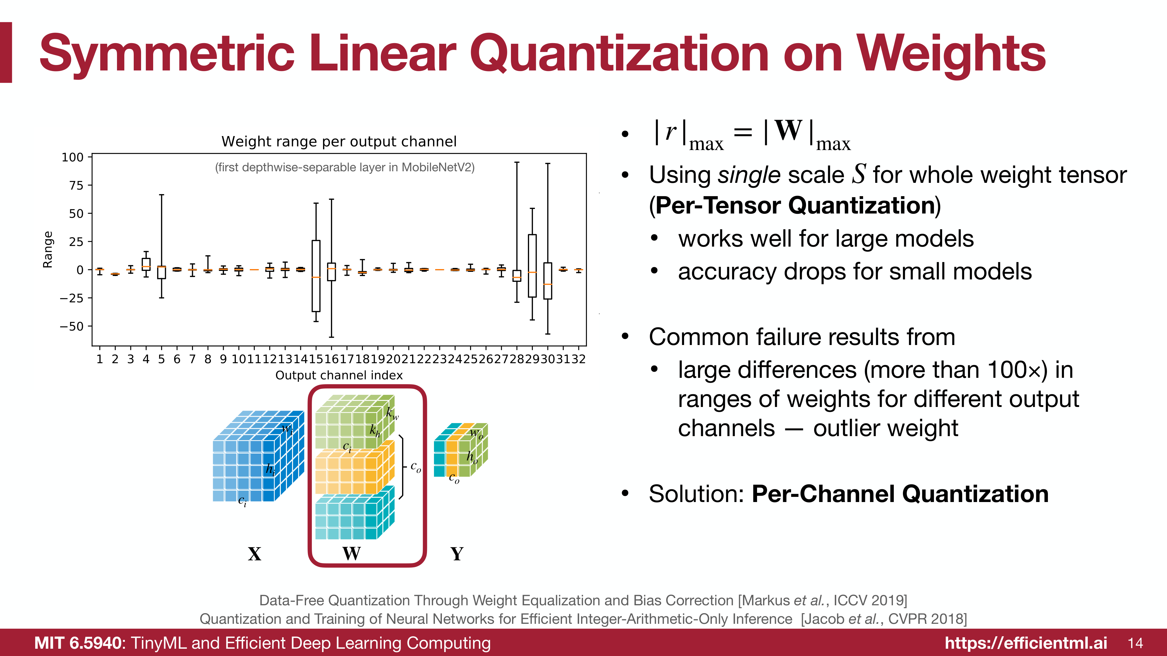 Weight ranges differ by 100× across channels—outliers in one channel destroy precision for all others
When channel 0 has weights in range $[-0.01, 0.01]$ but channel 50 spans $[-1.5, 1.5]$, a single scale factor wastes most of the quantization range for low-magnitude channels.
Per-Channel Quantization
The solution: use separate scale factors for each output channel.
For each output channel $i$:
\[S_{W,i} = \frac{\max(W[i, :, :, :]) - \min(W[i, :, :, :])}{q_{\max} - q_{\min}}\]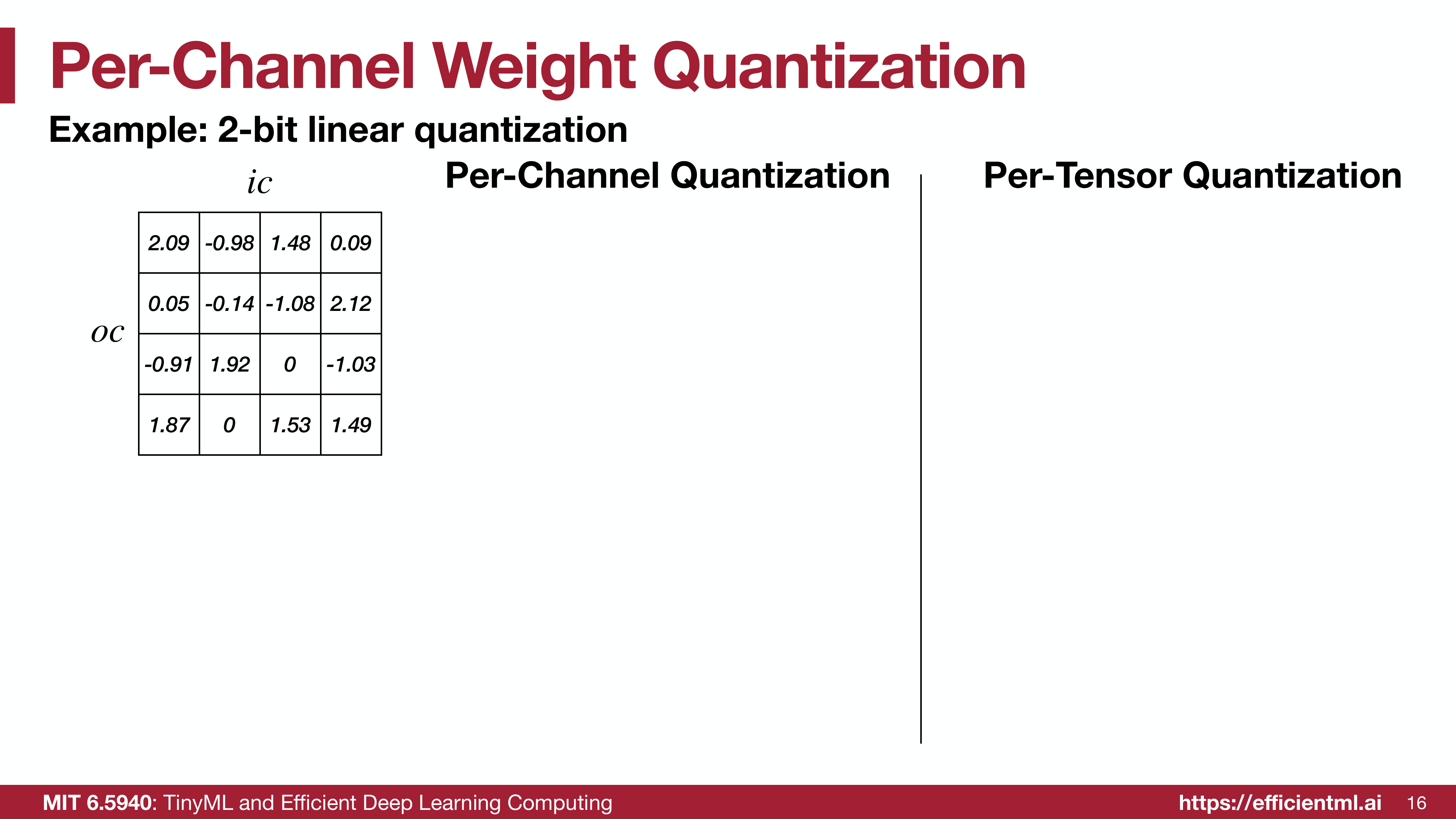 Per-channel quantization example with 2-bit linear quantization
Concrete example with 2-bit quantization:
Original weight matrix:
1
2
3
4
2.09  -0.98  1.48   0.09
0.05  -0.14 -1.08   2.12
-0.91  1.92  0.00  -1.03
1.87   0.00  1.53   1.49
| Per-tensor quantization ($ | r | _{\max} = 2.12$, $S = 2.12$): |
Reconstructed weights:
1
2
3
4
2.12   0.00  2.12   0.00
0.00   0.00 -2.12   2.12
0.00   2.12  0.00  -2.12
2.12   0.00  2.12   2.12
Reconstruction error: $|W - SqW|_F = 2.28$
Per-channel quantization (separate $S$ for each row):
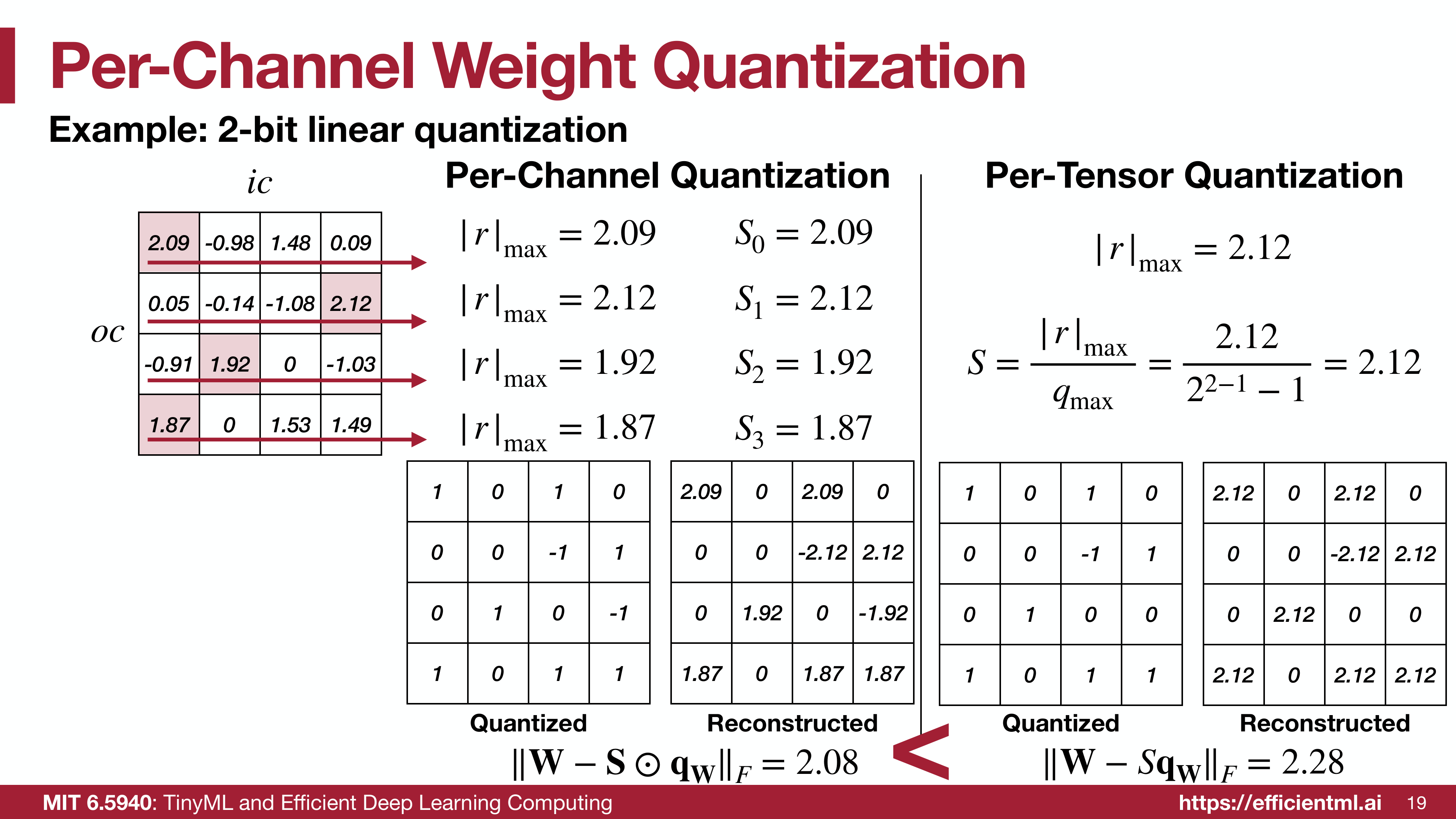 Per-channel quantization achieves better reconstruction with lower error
- Channel 0: $S_0 = 2.09$
- Channel 1: $S_1 = 2.12$
- Channel 2: $S_2 = 1.92$
- Channel 3: $S_3 = 1.87$
Reconstructed weights:
1
2
3
4
2.09   0.00  2.09   0.00
0.00   0.00 -2.12   2.12
0.00   1.92  0.00  -1.92
1.87   0.00  1.87   1.87
Reconstruction error: $|W - S \odot qW|_F = 2.08 < 2.28$
The per-channel approach reduces error by 8.8% in this example—a significant improvement that compounds across an entire network.
Group Quantization
Per-channel quantization works well for weights, but what about even finer granularity? Group quantization introduces hierarchical scaling with multiple levels:
\[r = (q - z) \cdot s_{l_0} \cdot s_{l_1} \cdot \ldots\]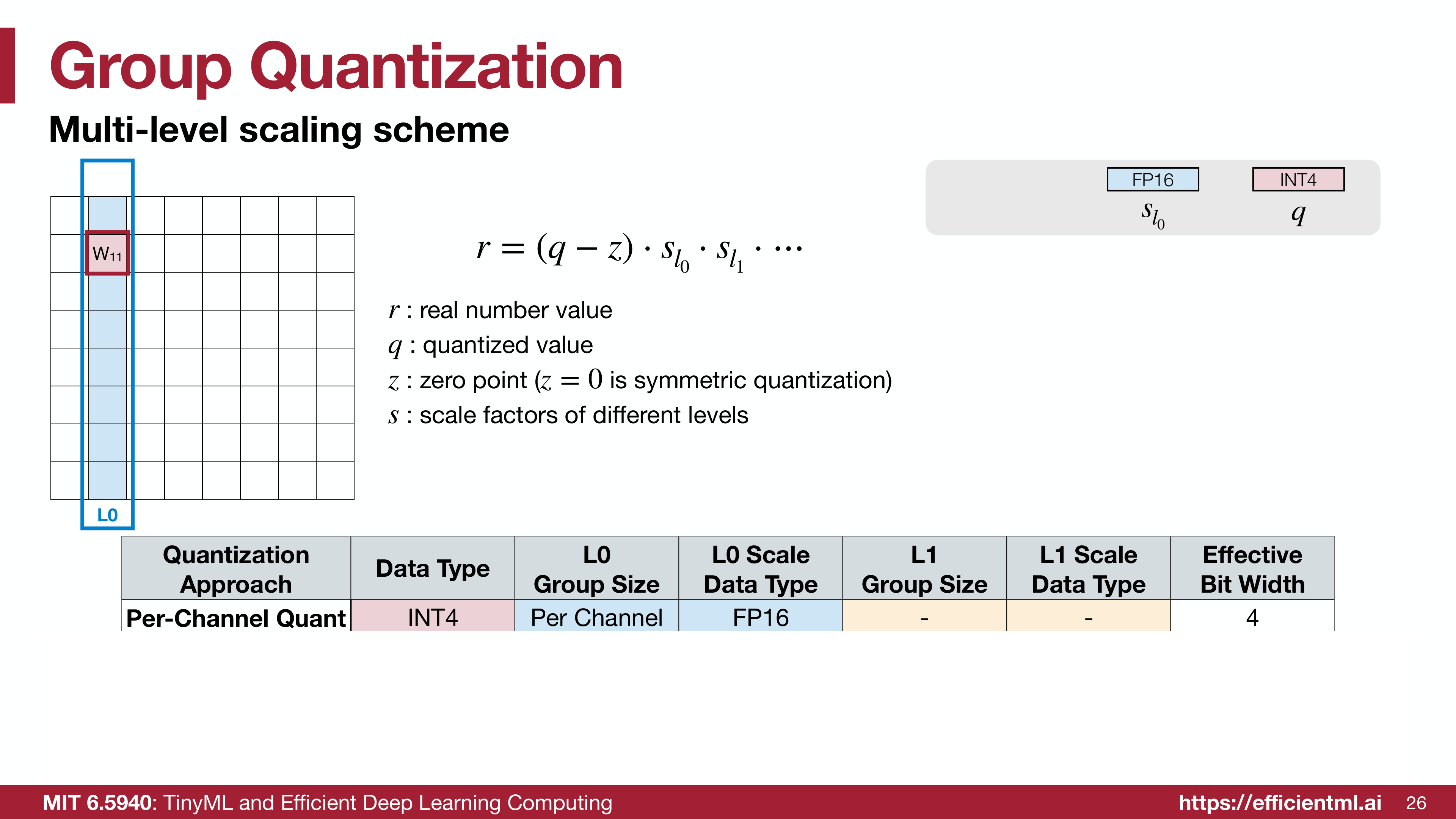 Multi-level scaling scheme balancing accuracy and efficiency
Key approaches:
VS-Quant (Per-Vector Scaled Quantization):
- Level 0: Integer scale factors per vector (e.g., every 16 elements)
- Level 1: Floating-point scale factor per tensor
- Effective bit-width: $4 + \frac{4}{16} = 4.25$ bits for 4-bit quantization
MX (Shared Micro-Exponent) Format:
- Level 0: Mantissa with shared exponent per small block (2 elements)
- Level 1: Shared exponent per larger block (16 elements)
- MX4: 3-bit mantissa + hierarchical exponents = 4 effective bits
- MX6: 5-bit mantissa + hierarchical exponents = 6 effective bits
The trade-off: slightly increased effective bit-width (4.25 vs 4.0 bits) for substantially better accuracy, especially for ultra-low precision quantization (FP4, INT4).
Hardware support: NVIDIA’s Blackwell GPUs include “micro-tensor scaling” for FP4, providing 2× throughput over FP8 while maintaining acceptable accuracy through group quantization.
Dynamic Range Clipping
Determining the floating-point range $[r_{\min}, r_{\max}]$ for activations poses a unique challenge: unlike weights (which are fixed), activation ranges vary across different inputs.
Exponential Moving Average (EMA)
During training or initial inference, track activation statistics using exponential moving average:
\[\hat{r}^{(t)}_{\max} = \alpha \cdot r^{(t)}_{\max} + (1 - \alpha) \cdot \hat{r}^{(t-1)}_{\max}\] \[\hat{r}^{(t)}_{\min} = \alpha \cdot r^{(t)}_{\min} + (1 - \alpha) \cdot \hat{r}^{(t-1)}_{\min}\]where $\alpha \in [0.01, 0.1]$ controls smoothing. This approach:
- Smooths observed ranges across thousands of training steps
- Reduces sensitivity to outliers
- Works well when integrated into training
Limitation: Requires access to training infrastructure and data.
Calibration-Based Methods
For true post-training quantization without training access, run a small calibration dataset (100-1000 samples) through the FP32 model and collect activation statistics.
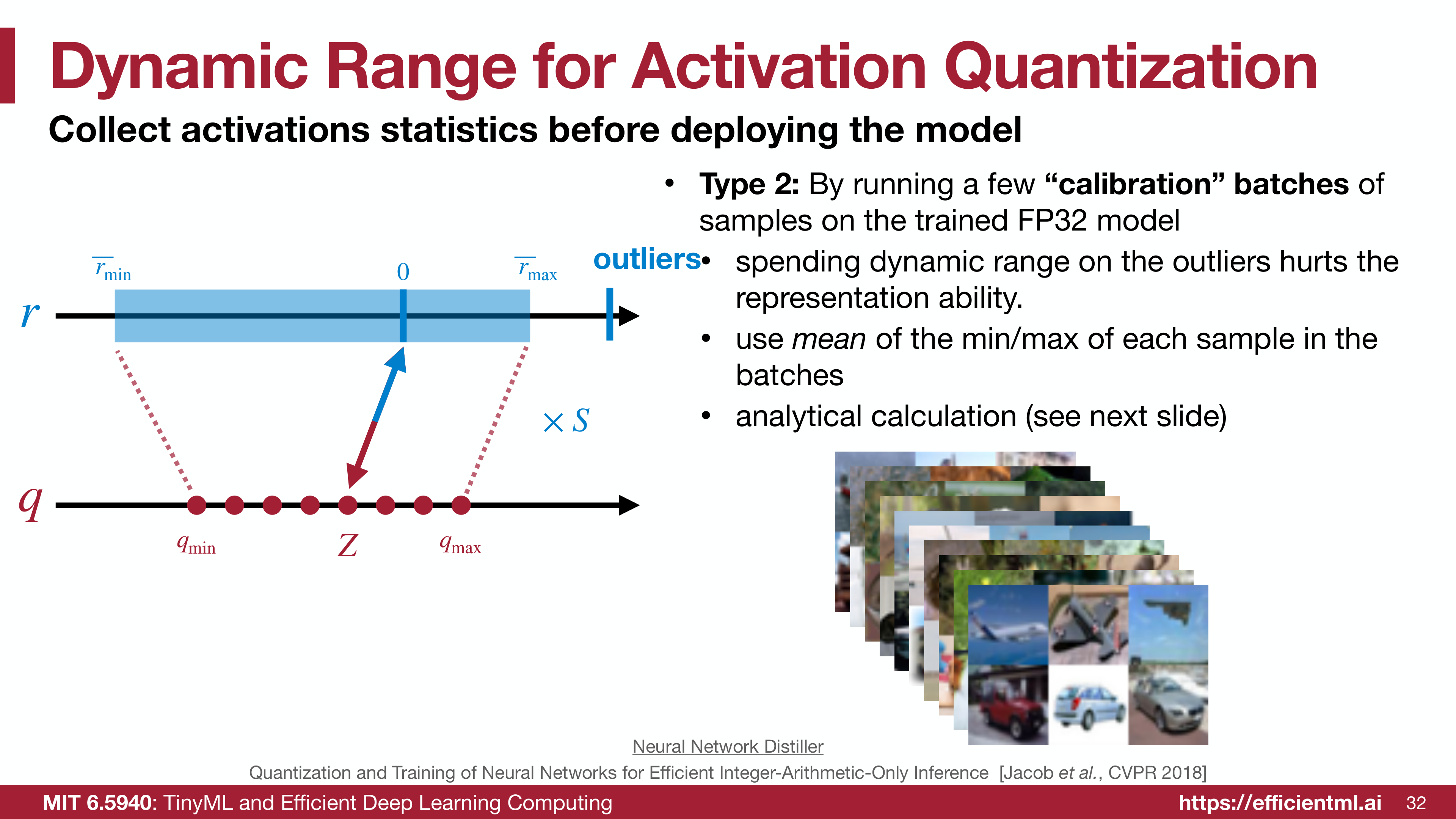 Spending dynamic range on outliers hurts representation—calibration identifies optimal clipping points
Three sophisticated approaches determine optimal clipping:
1. Mean-Square Error (MSE) Minimization
| Assume activations follow a specific distribution (Gaussian or Laplace) and find clipping threshold $ | r | _{\max}$ that minimizes: |
For Laplace distribution with parameter $b$:
\[|r|_{\max} = \begin{cases} 2.83b & \text{(2-bit)} \\ 3.89b & \text{(3-bit)} \\ 5.03b & \text{(4-bit)} \end{cases}\]The parameter $b$ is estimated from the calibration set’s empirical distribution. More advanced techniques like OCTAV use Newton-Raphson method for iterative refinement:
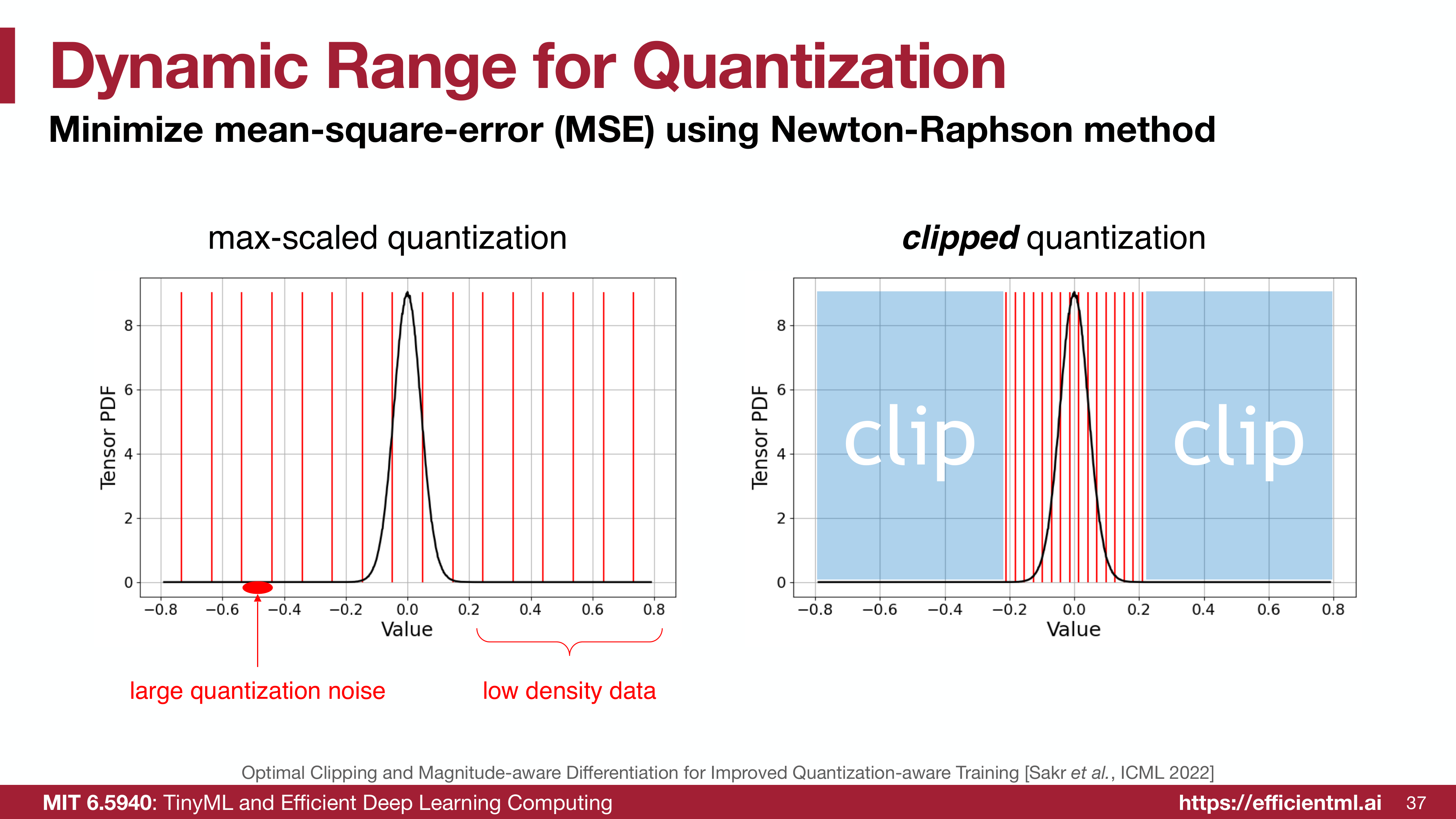 Optimal clipping reduces quantization noise in high-density regions
OCTAV results (INT4 quantization): | Network | FP32 Accuracy | OCTAV INT4 | |———|—————|————| | ResNet-50 | 76.07% | 75.84% | | MobileNet-V2 | 71.71% | 70.88% | | BERT-Large | 91.00% | 87.09% |
Only 0.23-0.83% accuracy loss for 8× model compression!
2. KL Divergence Minimization
Treat quantization as an information encoding problem. Minimize the Kullback-Leibler divergence between original and quantized activation distributions:
\[\min_{|r|_{\max}} D_{KL}(P \| Q) = \sum_i P(x_i) \log \frac{P(x_i)}{Q(x_i)}\]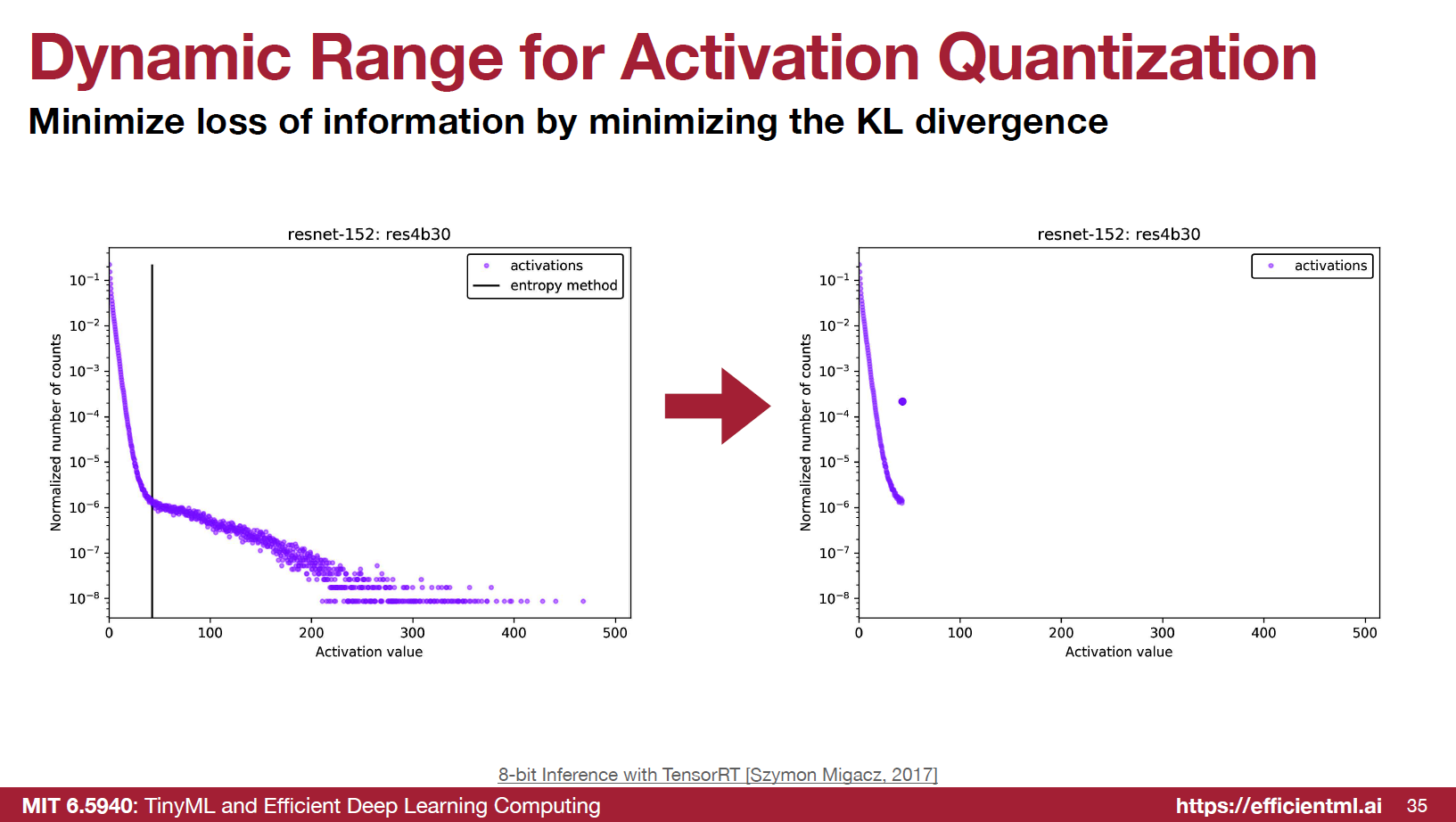 Finding clipping threshold that minimizes information loss
Algorithm:
- Collect activation histogram from calibration data
- For each candidate threshold:
- Quantize activations with that threshold
- Compute KL divergence between original and quantized distributions
- Select threshold with minimum KL divergence
This approach, popularized by TensorRT, works particularly well for CNNs where activation distributions are relatively smooth.
3. Percentile-Based Clipping
A simpler heuristic: use percentiles instead of absolute min/max:
\(r_{\max} = \text{percentile}(r, 99.9)\) \(r_{\min} = \text{percentile}(r, 0.1)\)
This automatically handles outliers without sophisticated optimization, though it may not be optimal.
Adaptive Rounding (AdaRound)
Traditional rounding-to-nearest isn’t optimal for weight quantization because weights are correlated—the best rounding for each weight individually isn’t the best rounding for the entire tensor collectively.
Philosophy: Round weights to values that best reconstruct the original activations, not the original weights themselves.
Problem formulation:
Instead of: \(\tilde{w} = \lfloor w \rceil\)
Choose from: \(\tilde{w} = \lfloor \lfloor w \rfloor + \delta \rceil, \quad \delta \in [0, 1]\)
Optimization objective:
\[\min_V \|Wx - \tilde{W}x\|^2_F + \lambda f_{\text{reg}}(V)\]where:
- $V$ is a learned variable (same shape as $W$)
- $h(V)$ maps $V$ to $(0,1)$ via rectified sigmoid
- $f_{\text{reg}}(V)$ encourages $h(V)$ to be binary (either 0 or 1)
Example scenario:
Original weights: [0.3, 0.5, 0.7, 0.2]
Rounding-to-nearest: [0, 1, 1, 0]
AdaRound (one potential result): [0, 0, 1, 0]
The second choice might better preserve the layer’s output distribution despite seemingly worse individual weight approximation.
Implementation: Run short-term optimization (typically 1000-5000 iterations) on calibration data with frozen activations. This is still “post-training” since it doesn’t require full dataset or extensive training.
PTQ Results on Real Networks
INT8 Quantization
| Network | FP32 | PTQ (Per-Tensor) | PTQ (Per-Channel) |
|---|---|---|---|
| GoogleNet | 70.2% | 69.75% (-0.45%) | 70.2% (0%) |
| ResNet-50 | 76.1% | 75.97% (-0.13%) | 75.5% (-0.6%) |
| ResNet-152 | 77.7% | 77.62% (-0.08%) | 75.9% (-1.8%) |
| MobileNet-V1 | 70.9% | - | 59.1% (-11.8%) |
| MobileNet-V2 | 71.9% | - | 69.8% (-2.1%) |
Observations:
- Large models (ResNet, GoogleNet) tolerate PTQ well with <1% accuracy loss
- Smaller models (MobileNets) with lower representational capacity suffer more
- Per-channel quantization essential for depth-separable convolutions
This motivates the need for quantization-aware training (Part 6) for aggressive quantization scenarios.
Practical PTQ Workflow
Step-by-Step Process
1. Prepare calibration dataset:
- Select 100-1000 representative samples
- Ensure coverage of different data modes/classes
- Use actual validation data if possible
2. Choose granularity strategy:
1
2
3
4
5
# Weights: Always per-channel
weight_quantization = "per-channel"

# Activations: Per-tensor usually sufficient
activation_quantization = "per-tensor"
3. Select calibration method:
1
2
3
4
5
# For CNNs: KL divergence
calibration_method = "kl_divergence"

# For transformers: MSE or percentile
calibration_method = "mse" or "percentile"
4. Apply AdaRound for weights:
1
2
# Optional but highly recommended for <8-bit
apply_adaround = True if target_bits < 8 else False
5. Validate and iterate:
- Check accuracy on validation set
- If accuracy unacceptable, try:
- Larger calibration set
- Different clipping method
- Per-channel for activations (higher overhead)
- Quantization-aware training (Part 6)
PyTorch Example
1
2
3
4
5
6
7
8
9
10
11
12
13
14
15
16
17
18
19
20
21
22
23
24
import torch
from torch.quantization import quantize_dynamic, quantize_static

# Load pretrained model
model = torchvision.models.resnet50(pretrained=True)
model.eval()

# Dynamic quantization (weights only, no calibration)
model_dynamic = quantize_dynamic(
    model,
    {torch.nn.Linear, torch.nn.Conv2d},
    dtype=torch.qint8
)

# Static quantization (weights + activations, requires calibration)
model.qconfig = torch.quantization.get_default_qconfig('fbgemm')
model_prepared = torch.quantization.prepare(model)

# Calibration
with torch.no_grad():
    for data in calibration_loader:
        model_prepared(data)

model_quantized = torch.quantization.convert(model_prepared)
When PTQ Falls Short
Post-training quantization works remarkably well for INT8 but struggles with:
Ultra-Low Precision (<8 bits)
At 4-bit or below, accuracy degradation becomes severe without training-time awareness. The model needs to learn quantization-friendly weight values.
Sensitive Architectures
- Transformers with attention mechanisms
- Models with batch normalization instability
- Networks with high activation variance
Deployment Constraints
- Hardware requiring specific quantization schemes
- Real-time inference with strict latency budgets
- Edge devices with limited calibration capability
In these scenarios, quantization-aware training (Part 6) becomes necessary.
Key Takeaways
- Post-training quantization converts trained FP32 models to INT8 without retraining
- Per-channel quantization dramatically improves accuracy for weights (especially depthwise-separable layers)
- Group quantization enables ultra-low precision (FP4/INT4) with hierarchical scaling
- Dynamic range clipping via KL divergence, MSE, or percentiles handles outliers effectively
- AdaRound optimizes weight rounding to preserve output distributions rather than weight values
- INT8 PTQ achieves <1% accuracy loss on large models like ResNet-50, GoogleNet
- Small models (MobileNets) require more sophisticated techniques or QAT
- Calibration dataset of 100-1000 samples typically sufficient for good results
Looking Ahead
Post-training quantization provides an excellent starting point for model compression, especially for INT8 deployment. However, when pushing to 4-bit or below, or when working with small models where every percentage point of accuracy matters, we need a more powerful approach.
Part 6 will explore Quantization-Aware Training (QAT), where the model learns to adapt to quantization constraints during training itself. By simulating quantization in the forward pass and using clever gradient estimation techniques, QAT recovers most accuracy loss from aggressive quantization—enabling 4-bit and even 2-bit models with minimal degradation.
Series Navigation:
- Part 1: Understanding Numeric Data Types
- Part 2: K-Means Based Weight Quantization
- Part 3: Linear Quantization Methods
- Part 4: Quantized Neural Network Operations
- Part 5: Post-Training Quantization Techniques (Current)
- Part 6: Quantization-Aware Training
- Part 7: Binary and Ternary Quantization
- Part 8: Mixed-Precision Quantization
References:
- MIT 6.5940: TinyML and Efficient Deep Learning Computing - EfficientML.ai Lecture 06: Quantization Part II (Fall 2024)
- Quantization and Training of Neural Networks for Efficient Integer-Arithmetic-Only Inference - Jacob et al., CVPR 2018
- Data-Free Quantization Through Weight Equalization and Bias Correction - Nagel et al., ICCV 2019
- 8-bit Inference with TensorRT - Szymon Migacz, GTC 2017
- Post-Training 4-Bit Quantization of Convolution Networks for Rapid-Deployment - Banner et al., NeurIPS 2019
- Up or Down? Adaptive Rounding for Post-Training Quantization - Nagel et al., ICML 2020
- Optimal Clipping and Magnitude-aware Differentiation for Improved Quantization-aware Training - Sakr et al., ICML 2022