Transformers from Scratch - Part 3: Multi-Head Attention Mechanism

In Part 2, we learned how Transformers convert text into meaningful embeddings with positional information. Now we’ll explore the heart of the Transformer: the attention mechanism.

The Core Innovation

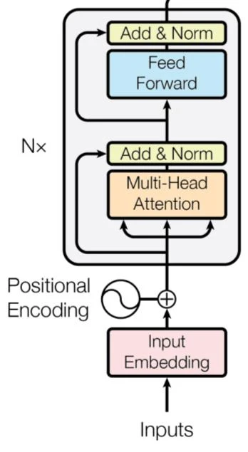
Multi-Head Attention is the core mechanism that makes Transformers so powerful. It allows the model to focus on different parts of the input sequence simultaneously, capturing various types of relationships and dependencies between words.

Understanding Attention: Query, Key, and Value

Before diving into multi-head attention, let’s understand the basic attention mechanism using an intuitive analogy.

The Library Analogy

Imagine you’re in a library looking for information:

1. Query (Q): What you’re looking for
   • “I need information about machine learning”
2. Key (K): Book titles/topics in the library
   • “Deep Learning Basics”
   • “Machine Learning Fundamentals”
   • “Cooking Recipes”
3. Value (V): The actual content of the books
   • The full text and information in each book

The attention mechanism:

• Compares your Query with all the Keys (book titles)
• Finds which Keys are most relevant
• Retrieves and combines the corresponding Values (book contents)

In Transformers

For each word in a sentence, attention helps answer: “Which other words should I pay attention to?”

Example: “The animal didn’t cross the street because it was too tired”

When processing “it”:

• Query: What does “it” refer to?
• Keys: Representations of all words in the sentence
• Values: Information content of all words
• Result: High attention to “animal” (it refers to the animal)

Scaled Dot-Product Attention

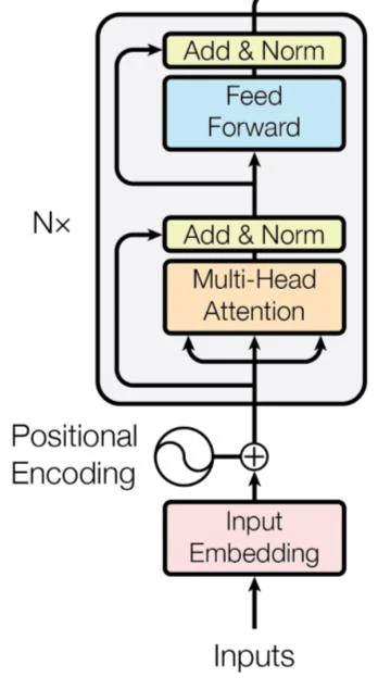
The fundamental building block of multi-head attention is scaled dot-product attention.

The Mathematical Formula

\[\text{Attention}(Q, K, V) = \text{softmax}\left(\frac{QK^T}{\sqrt{d_k}}\right)V\]

Let’s break this down step by step.

Step 1: Compute Similarity Scores

\[\text{Scores} = QK^T\]

• Multiply Query matrix with transpose of Key matrix
• Each element in the result represents how much a query “matches” with each key
• Higher score = more relevant

Dimensions:

• Q: (seq_len, d_k) - e.g., (10, 64)
• K^T: (d_k, seq_len) - e.g., (64, 10)
• Scores: (seq_len, seq_len) - e.g., (10, 10)

Example:

For sequence: "The cat sat"

Scores matrix:
           The   cat   sat
    The  [0.8   0.3   0.2]
    cat  [0.4   0.9   0.5]
    sat  [0.3   0.6   0.8]

Step 2: Scale by √d_k

\[\text{Scaled Scores} = \frac{QK^T}{\sqrt{d_k}}\]

Why scaling?

When $d_k$ (dimension of keys) is large, dot products can become very large in magnitude. This pushes the softmax function into regions where gradients are extremely small, making training difficult.

Example:

• If d_k = 64, we divide by √64 = 8
• This keeps the values in a reasonable range

Mathematical Insight:

• For random vectors, dot product grows with dimension
• Scaling by √d_k counteracts this growth
• Keeps gradients healthy during training

Step 3: Apply Softmax

\[\text{Attention Weights} = \text{softmax}\left(\frac{QK^T}{\sqrt{d_k}}\right)\]

Softmax converts scores to probabilities:

• All values between 0 and 1
• Sum to 1 for each query
• Larger scores get larger probabilities

Example:

Before softmax: [2.4, 1.2, 0.3]
After softmax:  [0.66, 0.24, 0.10]  (sum = 1.0)

Step 4: Weighted Sum of Values

\[\text{Output} = \text{Attention Weights} \times V\]

Multiply attention weights with values to get the final output.

• Each output is a weighted combination of all values
• Weights determined by attention scores
• Relevant values contribute more

Complete Example:

Input: "The cat sat"

Query for "cat":
1. Compute similarity with all words: [0.4, 0.9, 0.5]
2. Scale: [0.05, 0.11, 0.06] 
3. Softmax: [0.3, 0.5, 0.2]
4. Weighted sum:
   Output[cat] = 0.3 × Value[The] + 
                 0.5 × Value[cat] + 
                 0.2 × Value[sat]

Multi-Head Attention: Multiple Perspectives

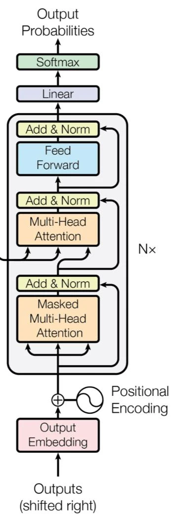
Instead of performing attention once, multi-head attention runs it multiple times in parallel, each with different learned projections.

Why Multiple Heads?

Different heads can focus on different aspects of relationships:

Example: “The animal didn’t cross the street because it was too tired”

• Head 1: Subject relationships
  • “it” → “animal” (what is “it”?)
• Head 2: Action-object relationships
  • “cross” → “street” (what is being crossed?)
• Head 3: Causality
  • “didn’t cross” → “tired” (why didn’t it cross?)

Single attention would average these, losing nuance. Multiple heads capture different patterns!

The Mathematical Formulation

\[\text{MultiHead}(Q, K, V) = \text{Concat}(head_1, ..., head_h)W^O\]

Each head is computed as:

\[head_i = \text{Attention}(QW^Q_i, KW^K_i, VW^V_i)\]

The Parameters

Weight matrices for each head $i$:

• $W^Q_i \in \mathbb{R}^{d_{model} \times d_k}$ - Query projection
• $W^K_i \in \mathbb{R}^{d_{model} \times d_k}$ - Key projection
• $W^V_i \in \mathbb{R}^{d_{model} \times d_v}$ - Value projection

Output projection:

• $W^O \in \mathbb{R}^{hd_v \times d_{model}}$ - Combines all heads

Typical values (from original paper):

• $h = 8$ attention heads
• $d_{model} = 512$ (model dimension)
• $d_k = d_v = 64$ (each head uses 512/8 = 64 dimensions)

Process Flow with Numbers

Let’s trace through with concrete dimensions:

Input: (seq_len, 512)

Step 1: Linear Projections for Each Head

For head i:
  Q_i = Q × W^Q_i → (seq_len, 64)
  K_i = K × W^K_i → (seq_len, 64)
  V_i = V × W^V_i → (seq_len, 64)

Step 2: Parallel Attention for 8 Heads

For each of 8 heads in parallel:
  head_i = Attention(Q_i, K_i, V_i) → (seq_len, 64)

Step 3: Concatenate All Heads

Concat(head_1, ..., head_8) → (seq_len, 512)
                                        ↑
                                8 heads × 64 = 512

Step 4: Final Linear Projection

Output = Concat × W^O → (seq_len, 512)

Result: Same shape as input (seq_len, 512), but now enriched with attention!

Dimension Flow Example

Input: "The cat sat" → 3 tokens

Starting shape: (3, 512)

After projection for each head:
  Q, K, V per head: (3, 64)

After attention per head:
  Each head output: (3, 64)

After concatenating 8 heads:
  (3, 8×64) = (3, 512)

After final projection:
  (3, 512)

Notice: Input and output have the same shape!

Self-Attention in the Encoder

In the encoder, we use self-attention where Q, K, and V all come from the same source (the previous layer’s output).

What this means:

• Each word attends to every word (including itself)
• Captures relationships within the input sentence
• All computed in parallel!

Example: “The cat sat on the mat”

For the word “cat”:

Query: cat's representation
Keys: [The, cat, sat, on, the, mat]
Values: [The, cat, sat, on, the, mat]

Result: cat's output considers all words

Benefits of Self-Attention

1. Parallel Processing

Unlike RNNs that process word-by-word:

RNN:  word1 → word2 → word3 → word4  (Sequential)
Attention: [word1, word2, word3, word4]  (Parallel)

Training speed: 100x faster on GPUs!

2. Long-Range Dependencies

Direct connection between any two words:

RNN path length from word 1 to word 100: 99 steps
Attention path length: 1 step (direct)

Result: Better at capturing long-distance relationships

3. Interpretability

We can visualize attention weights to see what the model focuses on:

When processing "it":
  Animal: 0.7 (high attention)
  Street: 0.2
  Cross: 0.1

This shows the model correctly identifies “it” refers to “animal”!

Practical Example: Complete Attention

Let’s work through a simple example:

Input: “Cat sat” (2 words)

Step 1: Embeddings (simplified to 4-dim)

cat: [1.0, 0.5, 0.2, 0.8]
sat: [0.3, 0.9, 0.7, 0.4]

Step 2: Project to Q, K, V (simplified to 2-dim per head)

Using learned weights W^Q, W^K, W^V:
Q: [[0.9, 0.3], [0.6, 0.8]]
K: [[0.8, 0.4], [0.5, 0.9]]
V: [[1.2, 0.7], [0.9, 1.1]]

Step 3: Compute Attention Scores

QK^T = [[0.9, 0.3], [0.6, 0.8]] × [[0.8, 0.5], [0.4, 0.9]]
     = [[0.84, 0.72], [0.80, 1.02]]

Step 4: Scale (d_k = 2, so √d_k = 1.41)

Scaled = [[0.60, 0.51], [0.57, 0.72]]

Step 5: Softmax

Attention weights:
  cat → [0.52, 0.48]  (52% to itself, 48% to "sat")
  sat → [0.46, 0.54]  (46% to "cat", 54% to itself)

Step 6: Weighted Sum

Output[cat] = 0.52 × V[cat] + 0.48 × V[sat]
            = 0.52 × [1.2, 0.7] + 0.48 × [0.9, 1.1]
            = [1.06, 0.89]

This output now contains information from both words!

What’s Next?

In Part 4, we’ll explore the remaining components of the encoder:

• Layer Normalization and why it’s crucial
• Feed-Forward Networks and their role
• Residual connections (Add & Norm)
• Complete encoder layer assembly

These components work together with attention to create the powerful encoder block.

Key Takeaways

1. Attention computes relationships between all positions simultaneously
2. Query, Key, Value are three projections that enable attention computation
3. Scaling by √d_k prevents gradient problems with large dimensions
4. Softmax converts scores to probability distributions
5. Multi-head attention captures different types of relationships in parallel
6. 8 heads each work with 64 dimensions (512/8) in the original Transformer
7. Self-attention allows each word to attend to all others including itself
8. Parallel processing makes training much faster than RNNs

---

Series Navigation:

• Part 1: From RNNs to Attention
• Part 2: Architecture and Embeddings
• Part 3: Multi-Head Attention Deep Dive (Current)
• Part 4: Layer Norm and Feed-Forward Networks
• Part 5: Decoder and Output Generation
• Part 6: Training, Inference, and Applications