Transformers from Scratch - Part 5: The Decoder and Output Generation

In Part 4, we completed our understanding of the encoder. Now let’s explore the decoder—the component that generates output sequences.

The Decoder: Overview

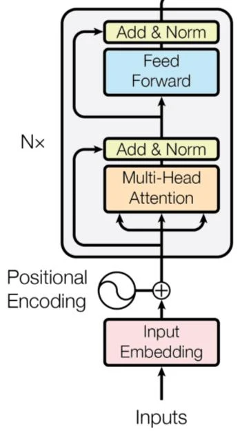
The decoder is similar to the encoder but with crucial differences. It generates the output sequence one token at a time in an autoregressive manner, using both:

• The encoder’s output
• Its own previous outputs

Three Sub-Layers

Each decoder layer has three sub-layers (encoder has two):

1. Masked Multi-Head Self-Attention
2. Cross-Attention (Encoder-Decoder Attention)
3. Position-wise Feed-Forward Network

Each sub-layer has residual connections + layer normalization.

Masked Multi-Head Self-Attention

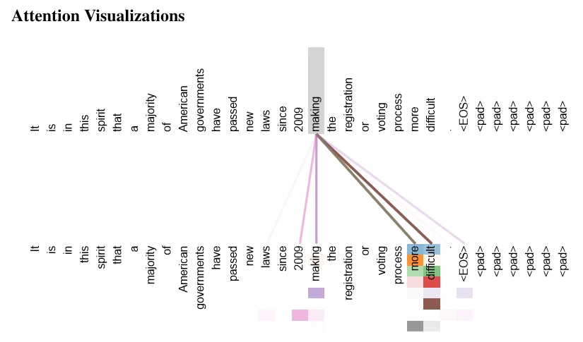
The first sub-layer uses masked self-attention—similar to encoder’s self-attention but with masking.

Why Masking?

The Problem: During training, we have access to the entire target sequence, but we must prevent positions from “cheating” by looking at future tokens.

Example: Translating “Hello” → “Bonjour”

When predicting position 2, the model should only see:

• Position 0 (start token)
• Position 1 (first output)
• NOT Position 2 (what we’re predicting!)
• NOT Positions 3, 4, … (future)

This preserves the autoregressive property: predicting position $i$ depends only on positions $< i$.

How Masking Works

Step 1: Create Mask Matrix

Create an upper triangular matrix of $-\infty$ values:

\[\text{Mask} = \begin{bmatrix} 0 & -\infty & -\infty & -\infty \\ 0 & 0 & -\infty & -\infty \\ 0 & 0 & 0 & -\infty \\ 0 & 0 & 0 & 0 \end{bmatrix}\]

Where:

• 0: Allow attention (can see)
• $-\infty$: Block attention (cannot see)

Step 2: Add to Attention Scores

Before softmax, add the mask:

\[\text{Attention}(Q, K, V) = \text{softmax}\left(\frac{QK^T}{\sqrt{d_k}} + \text{Mask}\right)V\]

Step 3: Softmax Effect

After adding mask:

Before softmax: [2.1, -∞, -∞, -∞]
After softmax:  [1.0, 0.0, 0.0, 0.0]  ← Future blocked!

The $-\infty$ values become 0 after softmax, effectively preventing attention to future positions.

Visual Example

Sentence: “I am learning transformers”

Position  Word          Can Attend To
   0      <START>       <START>
   1      I             <START>, I
   2      am            <START>, I, am
   3      learning      <START>, I, am, learning
   4      transformers  <START>, I, am, learning, transformers

Attention Matrix (1 = can see, 0 = blocked):

            <START>  I  am  learning  transformers
<START>        1     0   0      0          0
I              1     1   0      0          0
am             1     1   1      0          0
learning       1     1   1      1          0
transformers   1     1   1      1          1

The Formula

\[\text{MaskedAttention}(Q, K, V) = \text{softmax}\left(\frac{QK^T}{\sqrt{d_k}} + M\right)V\]

Where $M$ is the mask matrix that sets future positions to $-\infty$.

Complete Example

Input: “Cat sat” (generating translation)

Position 0 (predicting first word):

Attention scores: [0.9, -∞, -∞]
After softmax: [1.0, 0.0, 0.0]
← Can only attend to position 0 (self)

Position 1 (predicting second word):

Attention scores: [0.4, 0.8, -∞]
After softmax: [0.31, 0.69, 0.0]
← Can attend to positions 0 and 1

Position 2 (predicting third word):

Attention scores: [0.3, 0.5, 0.9]
After softmax: [0.15, 0.25, 0.60]
← Can attend to all three positions

Cross-Attention (Encoder-Decoder Attention)

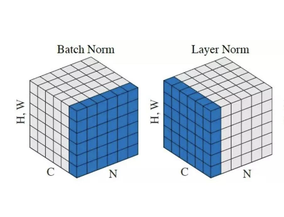
The second sub-layer is cross-attention—this is where the magic happens! The decoder attends to the encoder’s output.

How Cross-Attention Differs

Self-Attention: Q, K, V all from the same source

Q = K = V = previous layer output

Cross-Attention: Q from decoder, K and V from encoder

Q = decoder (what we're looking for)
K = encoder output (what's available)
V = encoder output (the information)

The Formula

\[\text{CrossAttention}(Q_{dec}, K_{enc}, V_{enc}) = \text{softmax}\left(\frac{Q_{dec}K_{enc}^T}{\sqrt{d_k}}\right)V_{enc}\]

Where:

• $Q_{dec}$: Query from previous decoder layer
• $K_{enc}$: Key from encoder output
• $V_{enc}$: Value from encoder output

Purpose of Cross-Attention

Cross-attention allows the decoder to focus on relevant parts of the input when generating each output token.

Machine Translation Example

Input (English): “I am a student” Output (French): “Je suis un étudiant”

When generating “étudiant”:

1. Decoder Query: “What input word should I focus on?”
2. Encoder Keys: Representations of [“I”, “am”, “a”, “student”]
3. Attention Computation:

   Query("étudiant") × Key("I"):       0.1 (low)
   Query("étudiant") × Key("am"):      0.1 (low)
   Query("étudiant") × Key("a"):       0.2 (low)
   Query("étudiant") × Key("student"): 0.9 (high!)
   

4. Softmax: [0.05, 0.05, 0.10, 0.80]
5. Weighted Sum: Heavily uses Value(“student”)

Result: The model correctly focuses on “student” to generate “étudiant”!

Visualization

Decoder Output    →    Encoder Input
"Je"              →    "I" (0.90 attention)
"suis"            →    "am" (0.85 attention)
"un"              →    "a" (0.88 attention)
"étudiant"        →    "student" (0.92 attention)

The cross-attention learns alignment between input and output!

Why This Works

1. Alignment Learning: Discovers which input words correspond to output words
2. Context Integration: Combines relevant input information for each output
3. Parallelizable: All decoder positions can attend to encoder simultaneously

Decoder Feed-Forward Network

The third sub-layer is identical to the encoder’s FFN:

\[\text{FFN}(x) = \text{ReLU}(xW_1 + b_1)W_2 + b_2\]

Same architecture:

• Expands: $512 → 2048$
• ReLU activation
• Projects back: $2048 → 512$

No differences from the encoder version!

Complete Decoder Layer

Putting all three sub-layers together:

\[\begin{align} z_1 &= \text{LayerNorm}(x + \text{MaskedMultiHeadAttention}(x, x, x)) \\ z_2 &= \text{LayerNorm}(z_1 + \text{CrossAttention}(z_1, \text{enc}, \text{enc})) \\ \text{output} &= \text{LayerNorm}(z_2 + \text{FFN}(z_2)) \end{align}\]

The Flow

Decoder Input (with position encoding)
    ↓
Masked Self-Attention
  (attend to previous positions only)
    ↓
Add & Norm
    ↓ (z1)
Cross-Attention
  Q from z1, K & V from encoder output
    ↓
Add & Norm
    ↓ (z2)
Feed-Forward Network
    ↓
Add & Norm
    ↓
Decoder Output

The Stack

Like the encoder, we stack 6 identical decoder layers:

Output Embedding + Positional Encoding
    ↓
Decoder Layer 1 (Masked Attn + Cross Attn + FFN)
    ↓
Decoder Layer 2 (Masked Attn + Cross Attn + FFN)
    ↓
...
    ↓
Decoder Layer 6 (Masked Attn + Cross Attn + FFN)
    ↓
Decoder Output (seq_len, 512)

Linear Layer and Softmax

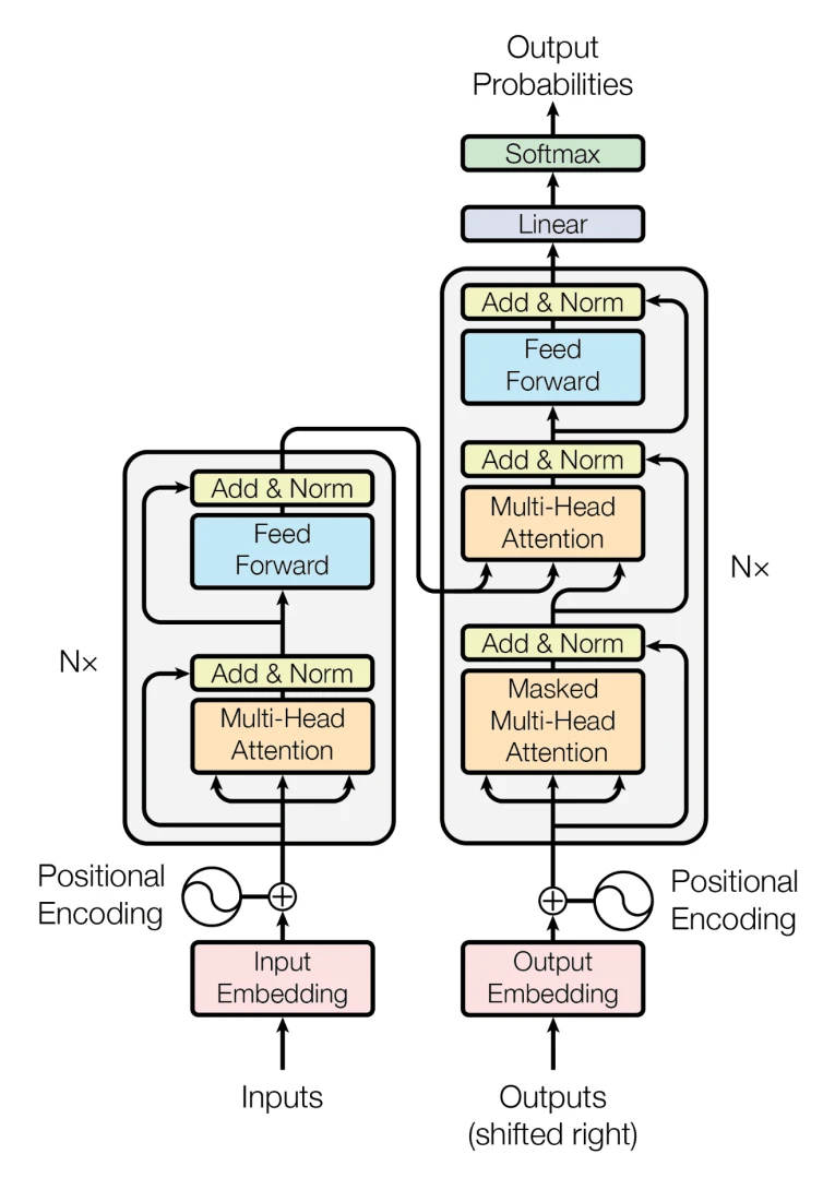
After the decoder stack, we need to convert decoder output into actual word predictions.

Linear Layer (Output Projection)

Projects from $d_{model}$ to vocabulary size:

\[\text{logits} = xW + b\]

Where:

• $x \in \mathbb{R}^{512}$: Decoder output
• $W \in \mathbb{R}^{512 \times V}$: Weight matrix
• $b \in \mathbb{R}^{V}$: Bias vector
• $V$: Vocabulary size (e.g., 30,000)
• $\text{logits} \in \mathbb{R}^{V}$: Raw scores

Dimensions:

Input:  (batch, seq_len, 512)
Output: (batch, seq_len, 30000)

Each position gets a score for every word in the vocabulary!

Softmax Layer

Converts raw scores to probabilities:

\[P(w_i) = \frac{e^{z_i}}{\sum_{j=1}^{V} e^{z_j}}\]

Properties:

1. All probabilities: $0 ≤ P(w_i) ≤ 1$
2. Sum to 1: $\sum_{i=1}^{V} P(w_i) = 1$
3. Higher scores → higher probabilities

Example

Logits for three words: $[2.0, 1.0, 0.1]$

Step 1: Exponentiate

e^2.0 = 7.39
e^1.0 = 2.72
e^0.1 = 1.11
Sum = 11.22

Step 2: Normalize

P("Bonjour") = 7.39 / 11.22 = 0.66 (66%)
P("Hello")   = 2.72 / 11.22 = 0.24 (24%)
P("Au")      = 1.11 / 11.22 = 0.10 (10%)

Result: Pick “Bonjour” (highest probability)

Output Generation During Inference

During inference, we generate one token at a time:

The Process

Step 1: Start Token

Input: <START>
Decoder: Processes <START>
Output: [0.7 for "Je", 0.2 for "Bonjour", ...]
Select: "Je"

Step 2: Use Previous Output

Input: <START> Je
Decoder: Processes both tokens
Output: [0.8 for "suis", 0.1 for "ai", ...]
Select: "suis"

Step 3: Continue

Input: <START> Je suis
Decoder: Processes all tokens
Output: [0.7 for "un", 0.2 for "le", ...]
Select: "un"

**Step 4: Repeat Until **

Input: <START> Je suis un étudiant
Decoder: Processes all tokens
Output: [0.9 for <END>, 0.05 for ".", ...]
Select: <END>

Selection Strategies

1. Greedy Decoding

Always pick the highest probability:

Pick: argmax(P(w))

Fast but can be suboptimal

2. Beam Search

Keep top-k candidates:

Beam width = 3:
  Path 1: "Je suis un étudiant" (score: 0.85)
  Path 2: "Je suis une étudiante" (score: 0.82)
  Path 3: "Je suis un élève" (score: 0.79)

Better quality, slower

3. Sampling

Sample from the probability distribution:

P("Je") = 0.6  → Randomly selected
P("Bonjour") = 0.3
P("Salut") = 0.1

More diverse outputs

Complete Translation Example

Input: “Hello world”

Step 1: Encoder processes "Hello world"
  → Encoder output: (2, 512)

Step 2: Decoder starts with <START>
  → Input: <START>
  → Masked attention: Can only see <START>
  → Cross-attention: Attends to encoder output
  → Output probability: P("Bonjour") = 0.8
  → Select: "Bonjour"

Step 3: Feed back prediction
  → Input: <START> Bonjour
  → Masked attention: Can see both tokens
  → Cross-attention: Attends to encoder output
  → Output probability: P("le") = 0.7
  → Select: "le"

Step 4: Continue
  → Input: <START> Bonjour le
  → Output: "monde"

Step 5: End
  → Input: <START> Bonjour le monde
  → Output: <END>

Final: "Bonjour le monde"

What’s Next?

In Part 6 (final part), we’ll explore:

• Training with teacher forcing
• Loss functions and optimization
• Inference strategies in detail
• Complete architecture summary
• Real-world applications
• Advantages over previous architectures

We’ll tie everything together and see how all the components work as a complete system!

Key Takeaways

1. Decoder has 3 sub-layers: Masked attention, cross-attention, feed-forward
2. Masked attention prevents looking at future tokens during training
3. Cross-attention connects decoder to encoder output
4. Q from decoder, K & V from encoder in cross-attention
5. Linear layer projects to vocabulary size
6. Softmax converts scores to probability distribution
7. Autoregressive generation: One token at a time
8. Beam search often better than greedy decoding
9. 6 decoder layers stacked like encoder

---

Series Navigation:

• Part 1: From RNNs to Attention
• Part 2: Architecture and Embeddings
• Part 3: Multi-Head Attention Deep Dive
• Part 4: Layer Norm and Feed-Forward Networks
• Part 5: Decoder and Output Generation (Current)
• Part 6: Training, Inference, and Applications