Transformers from Scratch - Part 4: Layer Norm and Feed-Forward Networks

In Part 3, we explored the multi-head attention mechanism. Now let’s understand the other crucial components that complete the encoder layer.

Recap: The Encoder Layer

Each encoder layer has two main sub-layers:

1. Multi-Head Self-Attention (covered in Part 3)
2. Feed-Forward Network (we’ll cover this today)

Both sub-layers are wrapped with:

• Residual connections (Add)
• Layer Normalization (Norm)

Layer Normalization

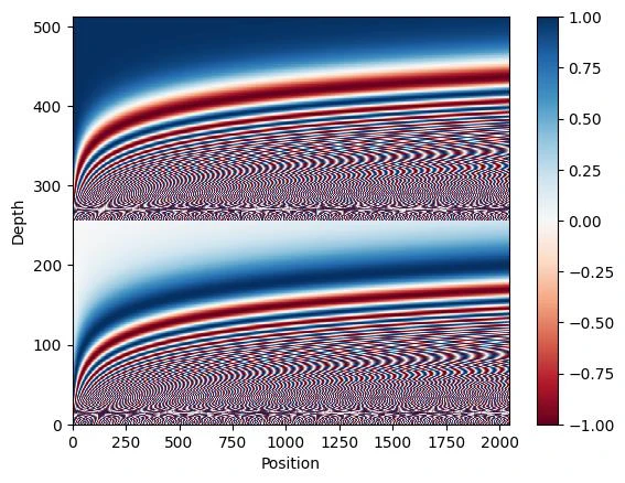
Layer Normalization is a technique that stabilizes and accelerates the training of deep neural networks. It’s applied after each sub-layer in the Transformer.

What is Layer Normalization?

Layer normalization normalizes the inputs across the features (not across the batch). For each sample, it computes the mean and variance across all features and normalizes.

The Mathematical Formula

\[\text{LayerNorm}(x) = \gamma \odot \frac{x - \mu}{\sqrt{\sigma^2 + \epsilon}} + \beta\]

Let’s break down each component:

Input vector: $x = [x_1, x_2, …, x_d]$ where $d$ is the feature dimension (512)

Mean across features: \(\mu = \frac{1}{d}\sum_{i=1}^{d} x_i\)

Variance across features: \(\sigma^2 = \frac{1}{d}\sum_{i=1}^{d} (x_i - \mu)^2\)

Normalize: \(\hat{x} = \frac{x - \mu}{\sqrt{\sigma^2 + \epsilon}}\)

Scale and shift: \(\text{LayerNorm}(x) = \gamma \odot \hat{x} + \beta\)

Where:

• $\gamma$ = Learnable scale parameter (initially 1)
• $\beta$ = Learnable shift parameter (initially 0)
• $\epsilon$ = Small constant for numerical stability (e.g., $10^{-6}$)
• $\odot$ = Element-wise multiplication

Step-by-Step Example

Let’s normalize a feature vector:

Input: $x = [2.0, 4.0, 6.0, 8.0]$

Step 1: Compute Mean \(\mu = \frac{2.0 + 4.0 + 6.0 + 8.0}{4} = 5.0\)

Step 2: Compute Variance \(\sigma^2 = \frac{(2-5)^2 + (4-5)^2 + (6-5)^2 + (8-5)^2}{4} = \frac{9+1+1+9}{4} = 5.0\)

Step 3: Normalize \(\hat{x} = \frac{[2, 4, 6, 8] - 5}{\sqrt{5.0 + 10^{-6}}} = \frac{[-3, -1, 1, 3]}{2.236} = [-1.34, -0.45, 0.45, 1.34]\)

Step 4: Scale and Shift (assuming $\gamma=1$, $\beta=0$ initially) \(\text{Output} = 1 \times [-1.34, -0.45, 0.45, 1.34] + 0 = [-1.34, -0.45, 0.45, 1.34]\)

Properties of the normalized output:

• Mean = 0
• Variance = 1
• Standard deviation = 1

Why Layer Normalization?

1. Training Stability

Without normalization, layer inputs can have wildly different scales:

Layer 1 output: [0.1, 0.2, 100.0, 0.3]  ← 100.0 dominates!

After normalization:

Layer 1 output: [-0.58, -0.57, 1.73, -0.57]  ← Balanced!

This keeps the distribution of activations consistent throughout training.

2. Faster Convergence

Normalized inputs lead to smoother loss landscapes:

• Gradients flow more smoothly
• Can use larger learning rates
• Networks train faster

Empirical observation: Training can be 2-3x faster with layer norm!

3. Reduces Internal Covariate Shift

During training, layer input distributions change as previous layers update. Layer norm minimizes this drift, making training more stable.

4. Works Well with Sequential Data

Unlike batch normalization:

• Independent of batch size: Works even with batch size = 1
• Same behavior in training and inference
• Perfect for variable-length sequences

Layer Norm vs Batch Norm

Aspect	Layer Normalization	Batch Normalization
Normalization Dimension	Across features (within sample)	Across batch (across samples)
Dependency	Independent of batch size	Requires reasonable batch size
Use Case	Sequential models, Transformers, NLP	CNNs, image processing
Training vs Inference	Same behavior	Different (uses running stats)
Variable Sequence Lengths	Handles naturally	Can be problematic

Example:

For input of shape (batch=2, features=4):

Batch: [[1, 2, 3, 4],
        [5, 6, 7, 8]]

Layer Norm: Normalize each row independently
  Row 1: [1,2,3,4] → normalized
  Row 2: [5,6,7,8] → normalized

Batch Norm: Normalize each column across batch
  Col 1: [1,5] → normalized
  Col 2: [2,6] → normalized
  Col 3: [3,7] → normalized
  Col 4: [4,8] → normalized

Residual Connections: Add & Norm

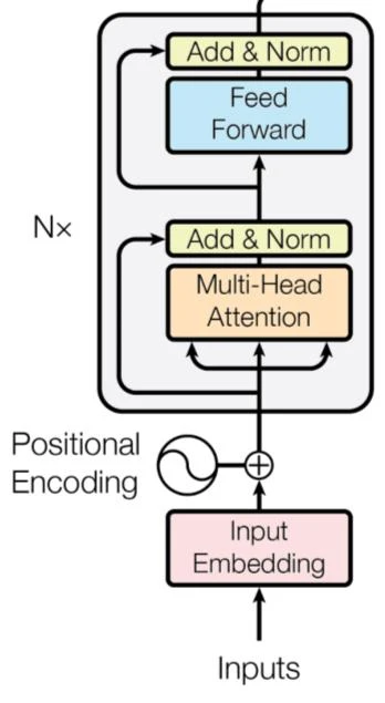
In Transformers, we use residual connections (Add) followed by Layer Normalization (Norm).

The Formula

\[\text{Output} = \text{LayerNorm}(x + \text{Sublayer}(x))\]

Where:

• $x$ = Input to the sub-layer
• $\text{Sublayer}(x)$ = Output of the sub-layer (e.g., attention or feed-forward)
• The + is element-wise addition

Why Residual Connections?

1. Gradient Flow

Residual connections create shortcuts for gradients:

Without residual:

Input → Layer1 → Layer2 → ... → Layer12 → Output
Gradients must flow back through all 12 layers

With residual:

Input ─────────────────────────────────────→ Output
  └→ Layer1 → Layer2 → ... → Layer12 ─────┘
Gradients can flow directly back (shortcut path!)

2. Prevents Degradation

Deep networks without residuals can perform worse than shallow ones (degradation problem). Residuals solve this:

Worst case: Layer learns identity function
  Sublayer(x) ≈ 0
  Output = x + 0 = x
  
Network can't get worse than shallow version!

3. Easier Optimization

The network learns residual functions (differences):

• Easier to learn small adjustments than entire transformations
• $\text{Sublayer}(x)$ learns what to add/change, not complete output

Complete Add & Norm Example

Input: $x = [1.0, 2.0, 3.0, 4.0]$

Sub-layer output: $\text{Sublayer}(x) = [0.5, -0.3, 0.2, 0.1]$

Step 1: Add (Residual) \(x + \text{Sublayer}(x) = [1.5, 1.7, 3.2, 4.1]\)

Step 2: Layer Norm

• Mean: $\mu = 2.625$
• Variance: $\sigma^2 = 1.359$
• Normalized: $[-0.97, -0.79, 0.49, 1.27]$

Final Output: $[-0.97, -0.79, 0.49, 1.27]$

Feed-Forward Network

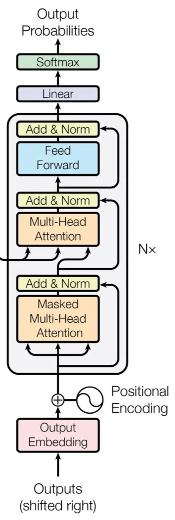
After attention, each encoder layer contains a Position-wise Feed-Forward Network. It’s a simple fully connected network applied to each position independently.

Architecture

Two linear transformations with ReLU activation:

\[\text{FFN}(x) = \text{ReLU}(xW_1 + b_1)W_2 + b_2\]

Or equivalently:

\[\text{FFN}(x) = \max(0, xW_1 + b_1)W_2 + b_2\]

The Parameters

Layer 1:

• $W_1 \in \mathbb{R}^{d_{model} \times d_{ff}}$ - Weight matrix
• $b_1 \in \mathbb{R}^{d_{ff}}$ - Bias vector

Layer 2:

• $W_2 \in \mathbb{R}^{d_{ff} \times d_{model}}$ - Weight matrix
• $b_2 \in \mathbb{R}^{d_{model}}$ - Bias vector

Dimensions (from original paper):

• $d_{model} = 512$ - Input/output dimension
• $d_{ff} = 2048$ - Hidden dimension (4× expansion!)

Process Flow

Step 1: Expand Dimensions

Input: (seq_len, 512)
After W1: (seq_len, 2048)

Example: [0.1, 0.2, ..., 0.5] (512 dims)
      → [0.3, -0.1, ..., 0.8] (2048 dims)

Step 2: Apply ReLU

ReLU(x) = max(0, x)

Before: [0.3, -0.1, 0.5, -0.2, ...]
After:  [0.3,  0.0, 0.5,  0.0, ...]  ← Negative values zeroed

Step 3: Project Back

After W2: (seq_len, 512)

[0.3, 0.0, 0.5, ...] (2048 dims)
→ [0.4, 0.2, ..., 0.6] (512 dims)

Why “Position-wise”?

The same FFN is applied to each position (word) independently:

For sequence "The cat sat":

Position 0 ("The"): FFN([...]) → [...]
Position 1 ("cat"): FFN([...]) → [...]  ← Same FFN!
Position 2 ("sat"): FFN([...]) → [...]

• Same weights ($W_1$, $W_2$) used for all positions
• Each position processed separately (no mixing)
• Equivalent to 1D convolution with kernel size 1

Purpose of Feed-Forward Network

1. Non-linear Transformation

Attention is largely linear. FFN adds non-linearity through ReLU:

Linear Attention → ReLU (non-linear) → Linear

Without this, the entire Transformer would be linear!

2. Feature Transformation

The 4× expansion ($512 → 2048$) provides more capacity:

• Learn complex feature combinations
• Process information gathered by attention
• 2048 intermediate features vs 512 output features

3. Information Processing

Think of it as “digest what attention found”:

• Attention: Gather relevant information
• FFN: Process and transform that information

Complete Example

Input vector: $x = [0.5, 1.0, -0.5, 0.3]$ (simplified to 4-dim)

Weights (simplified):

W1 = [[0.2, 0.3, 0.1],      (4 × 3 matrix)
      [0.4, -0.1, 0.5],
      [0.1, 0.2, -0.3],
      [-0.2, 0.4, 0.2]]
      
b1 = [0.1, -0.1, 0.2]

W2 = [[0.5, 0.2, -0.1, 0.3],   (3 × 4 matrix)
      [0.1, 0.4, 0.2, -0.2],
      [-0.3, 0.1, 0.5, 0.4]]
      
b2 = [0.0, 0.0, 0.0, 0.0]

Step 1: First Linear + Bias

xW1 + b1 = [0.5, 1.0, -0.5, 0.3] × W1 + b1
         = [0.47, 0.47, -0.09]

Step 2: ReLU

max(0, [0.47, 0.47, -0.09]) = [0.47, 0.47, 0.0]

Step 3: Second Linear + Bias

[0.47, 0.47, 0.0] × W2 + b2 = [0.28, 0.28, 0.05, 0.05]

Output: $[0.28, 0.28, 0.05, 0.05]$

Complete Encoder Layer

Now let’s put everything together!

The Two Sub-Layers

Sub-layer 1: Multi-Head Attention + Add & Norm \(z = \text{LayerNorm}(x + \text{MultiHeadAttention}(x, x, x))\)

Sub-layer 2: Feed-Forward + Add & Norm \(\text{output} = \text{LayerNorm}(z + \text{FFN}(z))\)

Complete Flow

Input: (seq_len, 512)
    ↓
Multi-Head Self-Attention
    ↓ (output: seq_len, 512)
Add with input (residual)
    ↓
Layer Normalization
    ↓ (z: seq_len, 512)
Feed-Forward Network
  → Expand to 2048
  → ReLU
  → Project to 512
    ↓ (output: seq_len, 512)
Add with z (residual)
    ↓
Layer Normalization
    ↓
Output: (seq_len, 512)

The Stack

The original Transformer uses 6 identical encoder layers stacked:

Input Embedding + Positional Encoding
    ↓
Encoder Layer 1 (Attention + FFN)
    ↓
Encoder Layer 2 (Attention + FFN)
    ↓
Encoder Layer 3 (Attention + FFN)
    ↓
Encoder Layer 4 (Attention + FFN)
    ↓
Encoder Layer 5 (Attention + FFN)
    ↓
Encoder Layer 6 (Attention + FFN)
    ↓
Encoder Output (seq_len, 512)

Each layer refines the representation!

What’s Next?

In Part 5, we’ll explore the decoder, which is more complex than the encoder:

• Masked Multi-Head Self-Attention
• Cross-Attention (Encoder-Decoder Attention)
• Output generation process
• Linear layer and softmax

The decoder uses similar components but with key modifications to generate output sequences.

Key Takeaways

1. Layer Normalization normalizes across features, stabilizing training
2. Residual connections enable gradient flow and prevent degradation
3. Add & Norm combines residual connections with layer normalization
4. Feed-Forward Network adds non-linearity and processes attention output
5. 4× expansion (512→2048→512) provides more representational capacity
6. Position-wise means same FFN applied to each position independently
7. Two sub-layers (Attention + FFN) both wrapped with Add & Norm
8. 6 encoder layers stacked to create deep representation

---

Series Navigation:

• Part 1: From RNNs to Attention
• Part 2: Architecture and Embeddings
• Part 3: Multi-Head Attention Deep Dive
• Part 4: Layer Norm and Feed-Forward Networks (Current)
• Part 5: Decoder and Output Generation
• Part 6: Training, Inference, and Applications