Efficiency Metrics Part 2: Memory Metrics for Deep Learning

In Part 1, we explored performance metrics. Now we’ll examine memory-related metrics—often the bottleneck in deep learning deployment, especially on mobile and edge devices.

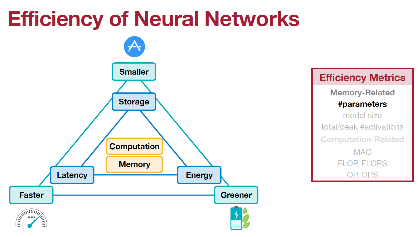
Memory metrics in the efficiency framework (Source: MIT 6.5940 Lecture 2)

Why Memory Metrics Matter

Memory is often the limiting factor, not computation. Understanding memory metrics helps you:

• Deploy models on resource-constrained devices (phones, IoT)
• Optimize cloud costs (memory costs money)
• Prevent out-of-memory errors during training
• Enable larger batch sizes for better throughput

Number of Parameters: The Model’s Knowledge Base

What Are Parameters? Parameters are the learned weights and biases in your neural network—the numbers that get adjusted during training.

Analogy: Think of parameters as the “knowledge” stored in the model. A book with more pages (parameters) contains more information but is heavier to carry around.

Definition: Parameters = total count of all weight and bias elements in the network

Parameter Count by Layer Type

Different layer types have different parameter counts:

Standard Notation:

Symbol	Meaning	Example
$C_i$	Input channels	3 (RGB)
$C_o$	Output channels	64 filters
$k_h, k_w$	Kernel height/width	3×3 filter
$g$	Number of groups	1 (standard)

Parameter Formulas:

Layer Type	Formula	Explanation
Linear (Fully Connected)	$C_o \times C_i$	Every input connects to every output
Standard Convolution	$C_o \times C_i \times k_h \times k_w$	Each output channel has $C_i$ kernels
Grouped Convolution	$\frac{C_o \times C_i \times k_h \times k_w}{g}$	Parameters divided across groups
Depthwise Convolution	$C_o \times k_h \times k_w$	One kernel per channel

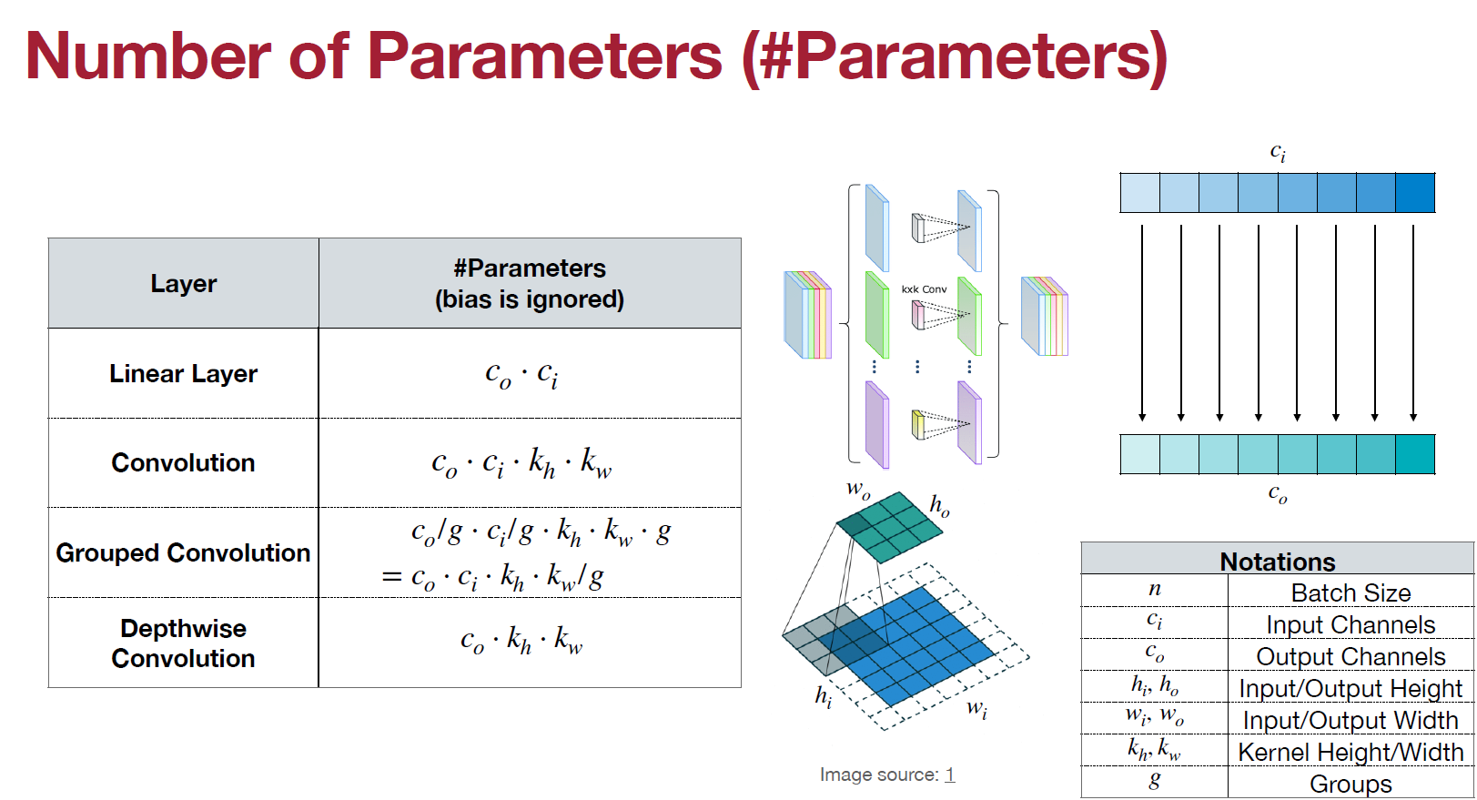
Complete parameter count formulas for different layer types (Source: MIT 6.5940 Lecture 2)

Concrete Examples

Example 1: Linear Layer

# Final classification layer
Input: 1000 features
Output: 10 classes

Parameters = C_o × C_i = 10 × 1,000 = 10,000 parameters

Example 2: Standard Convolution

# First layer of CNN
Input channels: 3 (RGB image)
Output channels: 64 (filters)
Kernel size: 3×3

Parameters = C_o × C_i × k_h × k_w
           = 64 × 3 × 3 × 3
           = 1,728 parameters

Example 3: Depthwise Separable Convolution

This efficiency technique is used in MobileNet:

Standard Conv:
  C_i=32, C_o=64, k=3×3
  Parameters = 64 × 32 × 3 × 3 = 18,432

Depthwise Separable:
  Depthwise: 32 × 3 × 3 = 288
  Pointwise: 64 × 32 × 1 × 1 = 2,048
  Total = 288 + 2,048 = 2,336
  
  Reduction: 18,432 → 2,336 (87% fewer parameters!)

Real Model Examples:

Model	Parameters	Use Case
SqueezeNet	1.2M	Mobile inference
MobileNetV2	3.5M	Efficient mobile CNN
ResNet-50	25.6M	Standard benchmark
VGG-16	138M	Classical deep network
GPT-3	175B	Large language model

Why Parameter Count Matters

Model Size: More parameters = more storage required Memory Bandwidth: More parameters to load from memory Training Time: More parameters = longer gradient computation Overfitting Risk: Too many parameters can overfit small datasets

Trade-off: Accuracy vs. Efficiency

• Fewer parameters: Faster, smaller, but may sacrifice accuracy
• More parameters: Better accuracy, but larger and slower

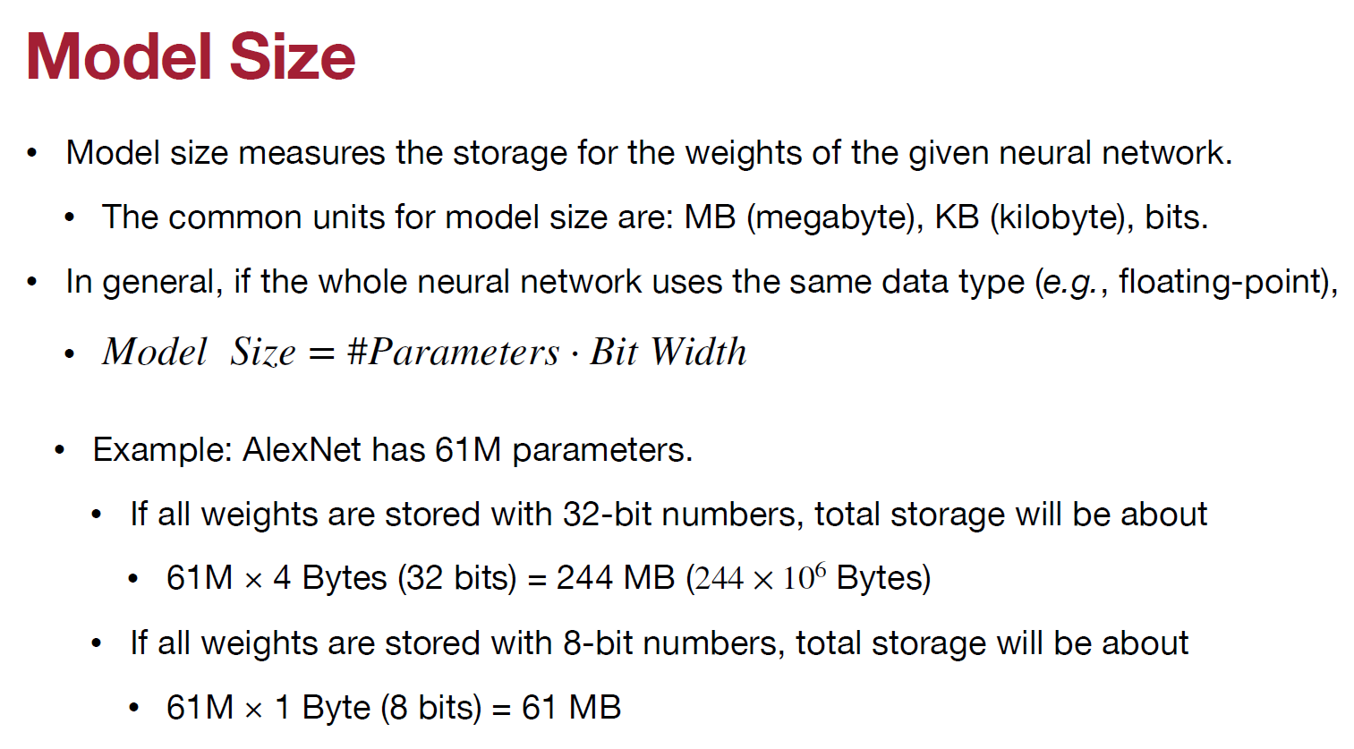
Model size depends on number of parameters and data type (Source: MIT 6.5940 Lecture 2)

Model Size: Storage Requirements

What is Model Size? The total amount of memory required to store the model’s parameters.

Formula:

\[\text{Model Size} = \text{Number of Parameters} \times \text{Bytes per Parameter}\]

Data Type Impact

Common Data Types:

Data Type	Bits	Bytes	Range	Typical Use
FP32	32	4	High precision	Training
FP16	16	2	Medium precision	Inference
INT8	8	1	Quantized	Edge devices
INT4	4	0.5	Highly quantized	Extreme compression

Concrete Examples

Example: AlexNet (61M parameters)

FP32 (32 bits):
  61M × 4 bytes = 244 MB

FP16 (16 bits):
  61M × 2 bytes = 122 MB (50% reduction)

INT8 (8 bits):
  61M × 1 byte = 61 MB (75% reduction)

Example: GPT-3 (175B parameters)

FP32:
  175B × 4 bytes = 700 GB

FP16:
  175B × 2 bytes = 350 GB

INT8:
  175B × 1 byte = 175 GB

Why This Matters: GPT-3 in FP32 doesn’t fit on a single GPU (A100 has 80GB). Requires model parallelism or quantization.

Practical Implications

Mobile Deployment:

Typical phone app size limit: ~100 MB
ResNet-50 (FP32): 98 MB → Fits (barely)
ResNet-50 (INT8): 25 MB → Fits comfortably + room for app

Cloud Cost:

AWS storage: $0.023/GB/month

Store 1000 ResNet-50 models:
  FP32: 98 GB × $0.023 = $2.25/month
  INT8: 25 GB × $0.023 = $0.58/month
  
Annual savings: ($2.25 - $0.58) × 12 = $20/year per 1000 models

Activation Memory: The Hidden Cost

What are Activations? Activations are the intermediate outputs produced by each layer during forward pass. During training, they must be stored for backpropagation.

Why Activations Matter:

• Training: Must store all activations for gradient computation
• Inference: Only need current layer’s output (much smaller)
• Memory Bottleneck: Often larger than model parameters

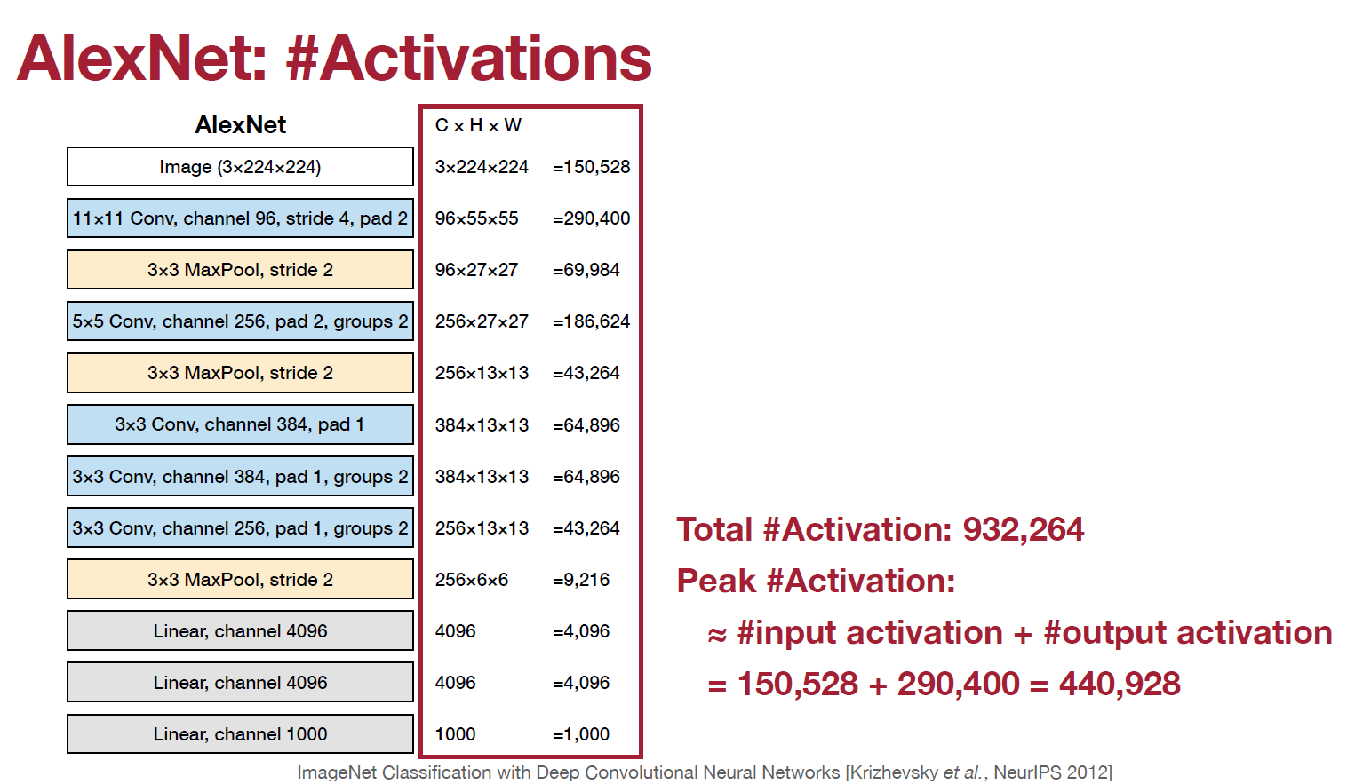
Total Activations

Definition: Overall memory needed to store all intermediate outputs as data moves through the network.

Formula for Convolutional Layer:

\[\text{Activation Memory} = n \times C_o \times h_o \times w_o \times \text{bytes per value}\]

Where:

• $n$ = batch size
• $C_o$ = output channels
• $h_o, w_o$ = output height and width

Concrete Example: ResNet-50

Input: 224×224×3 RGB image
Batch size: 32
Data type: FP32 (4 bytes)

Layer 1 (Conv): 32 × 64 × 112 × 112 × 4 = 161 MB
Layer 2 (Conv): 32 × 64 × 56 × 56 × 4 = 40 MB
...
Total activations: ~5 GB for batch of 32

Key Insight: Activation memory grows linearly with batch size. This is why you can’t always use arbitrarily large batches—you’ll run out of GPU memory.

Peak Activations

Definition: Maximum memory needed at any single point during execution.

Why It Matters: This determines minimum GPU memory required. If peak exceeds available memory, training fails with OOM (Out Of Memory) error.

Example: U-Net Architecture

Encoder path (downsampling):
  Memory increases as channels grow
  
Bottleneck:
  Peak memory usage (largest feature maps)
  
Decoder path (upsampling):
  Memory decreases as resolution grows
  
Skip connections:
  Must keep encoder activations in memory
  Increases peak significantly

Memory Optimization Strategies

1. Gradient Checkpointing

Trade-off: Memory for computation

Without checkpointing:
  Store all activations: 5 GB memory
  Forward + backward: 100 ms

With checkpointing:
  Store only checkpoints: 1 GB memory (80% reduction)
  Forward + recompute + backward: 150 ms (50% slower)

When to Use: When memory is the bottleneck, not compute speed.

2. Mixed Precision Training

FP32 training:
  Activations: 32 bits per value
  Memory: High

Mixed Precision (FP16 + FP32):
  Activations: 16 bits per value
  Memory: 50% reduction
  Speed: 2-3× faster (Tensor Cores)

3. Smaller Batch Sizes

Batch 64:
  Activation memory: 10 GB
  Training time: 2 hours
  
Batch 32:
  Activation memory: 5 GB (fits on GPU!)
  Training time: 3 hours (still completes)

Practical Memory Budget Example

Scenario: Train ResNet-50 on NVIDIA V100 (16GB memory)

Memory Breakdown:

Model parameters (FP32):        98 MB    (0.6%)
Optimizer state (Adam):        196 MB    (1.2%)
Gradients:                      98 MB    (0.6%)
Activations (batch=32):      5,000 MB   (31.3%)
Framework overhead:          1,000 MB    (6.3%)
Available buffer:            9,608 MB   (60%)
─────────────────────────────────────────────
Total used:                  6,392 MB   (40%)

Result: Can fit batch size 32 comfortably. Could potentially increase to 48-64.

Key Takeaways

Parameters Define Model Capacity: More parameters = more learned knowledge, but also more storage and computation.

Model Size is Flexible: Same model can be stored in different precisions (FP32, FP16, INT8) with 2-4× size differences.

Activations Dominate Training Memory: During training, activation memory often exceeds parameter memory by 10-50×.

Peak Memory Determines Feasibility: You need enough memory for peak activation, not average. This determines maximum batch size.

Optimization Strategies Exist: Gradient checkpointing, mixed precision, and smaller batches can reduce memory requirements significantly.

What’s Next?

In Part 3, we’ll explore computation metrics: MACs, FLOPs, and how to calculate the actual computational cost of different layer types.

---

Series Navigation:

• Part 1: Performance Metrics
• Part 2: Memory Metrics (Current)
• Part 3: Computation Metrics

References:

• MIT 6.5940: TinyML and Efficient Deep Learning Computing (Fall 2024)
• Efficient Processing of Deep Neural Networks - Sze et al., Synthesis Lectures on Computer Architecture 2020
• Mixed Precision Training - Micikevicius et al., ICLR 2018