GPU Memory Hierarchy Part 3: Optimization and Best Practices

In Part 1 and Part 2, we explored the GPU memory hierarchy. Now we’ll dive into practical optimization strategies and performance measurement.

Memory Bandwidth: The Hidden Bottleneck

Understanding the Roofline Model:

GPU performance is limited by either:

1. Compute Bound: Limited by FLOPS capacity
2. Memory Bound: Limited by memory bandwidth

A100 Specifications:

• Peak Compute: 312 TFLOPS (FP16 with Tensor Cores)
• Memory Bandwidth: 1555 GB/s

Arithmetic Intensity: \(\text{Arithmetic Intensity} = \frac{\text{FLOPs}}{\text{Bytes Transferred}}\)

Example: Matrix Multiplication: For $C = A \times B$ where $A, B, C$ are $N \times N$ matrices:

• FLOPs: $2N^3$ (multiply-add operations)
• Bytes: $3N^2 \times 4$ bytes (loading A, B, writing C in FP32)
• Arithmetic Intensity: $\frac{2N^3}{12N^2} = \frac{N}{6}$

For N=1024:

• Arithmetic Intensity = 170 FLOPs/byte
• This is compute-bound (good for GPUs)

For N=64:

• Arithmetic Intensity = 10 FLOPs/byte
• This is memory-bound (optimization needed)

Key Insight: Small matrix multiplications (common in batch size 1 inference) are memory-bound, not compute-bound. Optimizing memory access is more important than adding more compute.

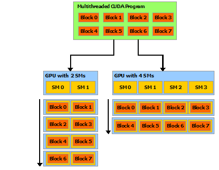
GPU performance scaling with workload size (Source: NVIDIA CUDA Programming Guide)

Five Essential Optimization Techniques

1. Minimize Global Memory Transfers

Bad Pattern:

for i in range(num_layers):
    x = layer[i](x)  # Each layer reads/writes to global memory

Good Pattern (Operator Fusion):

x = fused_layers(x)  # Multiple operations fused, fewer memory round-trips

Speedup: 2-3×

Why It Works: Each layer typically performs relatively few operations per byte of data. Fusing layers keeps intermediate results in faster memory (registers/shared memory) instead of writing to and reading from global memory.

2. Maximize Data Reuse in Shared Memory

Tiled Matrix Multiplication:

__global__ void matmul_tiled(float *A, float *B, float *C, int N) {
    __shared__ float tileA[TILE_SIZE][TILE_SIZE];
    __shared__ float tileB[TILE_SIZE][TILE_SIZE];
    
    // Load tile once, reuse TILE_SIZE times
    for (int tile = 0; tile < N/TILE_SIZE; tile++) {
        tileA[ty][tx] = A[...];  // Shared memory load
        tileB[ty][tx] = B[...];
        __syncthreads();
        
        // Reuse data in shared memory
        for (int k = 0; k < TILE_SIZE; k++) {
            sum += tileA[ty][k] * tileB[k][tx];
        }
    }
}

Benefit: Load data once from global memory (200-400 cycles), reuse many times from shared memory (4-8 cycles). For TILE_SIZE=16, this provides ~20× speedup.

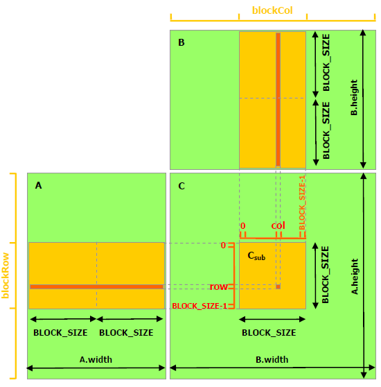
Tiled matrix multiplication strategy for data reuse (Source: NVIDIA CUDA Programming Guide)

3. Coalesce Memory Accesses

Uncoalesced (Slow):

# Strided access pattern
for i in range(N):
    x[i * stride] = value  # Causes multiple memory transactions

Coalesced (Fast):

# Contiguous access pattern
for i in range(N):
    x[i] = value  # Single memory transaction for multiple threads

Speedup: 5-10×

Why It Matters: The GPU memory system groups threads into warps (32 threads). When all threads in a warp access consecutive memory locations, the GPU can combine these into a single memory transaction.

4. Use Mixed Precision Training

FP32 (Standard):

• 4 bytes per parameter
• 1555 GB/s → 388B parameters/second

FP16 (Half Precision):

• 2 bytes per parameter
• 1555 GB/s → 776B parameters/second

Speedup: 2× memory bandwidth efficiency

Additional Benefits:

• Smaller memory footprint (fit larger models)
• Faster tensor core operations
• Only minimal accuracy loss with proper loss scaling

5. Enable Persistent Kernels

Keep data in faster memory across kernel launches:

# Traditional: Data moves to global memory between kernels
output1 = kernel1(input)  # Write to global memory
output2 = kernel2(output1)  # Read from global memory

# Persistent kernel: Data stays in cache/shared memory
output = fused_kernel(input)  # No intermediate global memory transfer

Speedup: 2-4× for multi-stage operations

Memory Hierarchy and Model Architecture Design

Design Principle: Architecture choices should be informed by memory hierarchy constraints.

Example 1: Attention Mechanism Memory Footprint

Standard Attention: \(\text{Memory} = O(N^2) \text{ for attention matrix}\)

For sequence length $N=1024$:

• Attention matrix: $1024^2 \times 4$ bytes = 4 MB (fits in L2 cache)

For sequence length $N=16384$:

• Attention matrix: $16384^2 \times 4$ bytes = 1 GB (exceeds cache, lives in global memory)

Solution: Sparse attention, Flash Attention (memory-efficient algorithms that reduce memory from $O(N^2)$ to $O(N)$).

Example 2: Batch Size Selection

Small Batch (Batch Size = 1):

• Low arithmetic intensity
• Memory-bound
• GPU underutilized

Large Batch (Batch Size = 256):

• High arithmetic intensity
• Compute-bound
• GPU well-utilized

Optimal Batch Size: Balance memory capacity and arithmetic intensity. For A100, typically 32-256 depending on model size.

Measuring Memory Performance

Tool 1: NVIDIA Nsight Compute

ncu --metrics dram__bytes_read,dram__bytes_write python train.py

Key Metrics:

• dram__bytes_read: Bytes read from HBM
• dram__bytes_write: Bytes written to HBM
• l2_cache_hit_rate: L2 cache effectiveness
• sm__sass_average_data_bytes_per_sector: Memory access efficiency

Interpreting Results:

• L2 cache hit rate >70%: Good temporal locality
• L2 cache hit rate <30%: Poor memory access patterns
• Bytes per sector <50%: Uncoalesced accesses

Tool 2: PyTorch Profiler

with torch.profiler.profile(
    activities=[torch.profiler.ProfilerActivity.CUDA],
    with_stack=True
) as prof:
    model(input)

print(prof.key_averages().table(sort_by="cuda_memory_usage"))

What to Look For:

• Operations with high memory usage
• Memory allocation patterns
• Kernel execution time vs memory transfer time

Tool 3: Memory Bandwidth Utilization

achieved_bandwidth = (bytes_transferred / elapsed_time)
memory_bandwidth_utilization = achieved_bandwidth / peak_bandwidth_HBM

# Goal: >70% utilization for memory-bound kernels

Bandwidth Efficiency:

• 80%: Excellent - memory system well-utilized

• 50-80%: Good - room for improvement
• <50%: Poor - likely uncoalesced accesses or small operations

Common Pitfalls and Solutions

Pitfall 1: Register Spilling

Problem: Using too many variables causes register spilling to slow local memory.

Solution: Reduce variable scope, use compiler flags to increase register allocation, or restructure code.

Pitfall 2: Bank Conflicts in Shared Memory

Problem: Multiple threads accessing the same shared memory bank simultaneously.

Solution: Pad arrays to avoid conflicts or restructure access patterns.

// Bad: Bank conflicts
__shared__ float data[32][32];

// Good: Padded to avoid conflicts
__shared__ float data[32][33];  // Extra column eliminates conflicts

Pitfall 3: Ignoring Cache Behavior

Problem: Accessing data in patterns that defeat cache.

Solution: Structure loops for temporal and spatial locality. Access data in the order it’s stored in memory.

Practical Checklist for Memory Optimization

Before Coding:

• Calculate arithmetic intensity for your operation
• Determine if compute-bound or memory-bound
• Plan data reuse strategy

During Implementation:

• Use mixed precision where possible
• Coalesce memory accesses
• Utilize shared memory for frequently reused data
• Fuse operations to reduce memory round-trips

After Implementation:

• Profile with Nsight Compute
• Measure memory bandwidth utilization
• Check L2 cache hit rates
• Verify coalesced access patterns

Key Takeaways

Memory Bottleneck Reality: Modern GPUs are often memory-bound, not compute-bound. A 10× improvement in memory efficiency can outweigh a 2× increase in compute power.

Optimization Priority: Focus on minimizing global memory accesses first (operator fusion), then maximize data reuse (tiling), then ensure coalesced accesses.

Tools Matter: Use profiling tools (Nsight Compute, PyTorch Profiler) to identify bottlenecks. Don’t guess - measure.

Arithmetic Intensity: Understanding the roofline model helps predict whether your kernel is compute-bound or memory-bound, guiding optimization efforts.

Energy Efficiency: Memory-efficient algorithms are also energy-efficient. Moving data costs 100× more energy than computation.

What’s Next?

Continue exploring related topics:

• Flash Attention: Memory-efficient attention algorithms
• Model Quantization: Reduce memory footprint and bandwidth requirements
• Neural Network Pruning: Decrease model size to fit in faster memory tiers
• Tensor Core Programming: Leverage specialized hardware for mixed-precision compute
• CUDA Programming: Write custom kernels optimized for memory hierarchy

Deep Dive Resources:

• NVIDIA CUDA C++ Programming Guide: Memory Hierarchy sections
• “Making Deep Learning Go Brrrr From First Principles” by Horace He
• NVIDIA Nsight Compute Documentation: Memory profiling tutorials

---

Series Navigation:

• Part 1: Understanding the Hierarchy
• Part 2: Global and Specialized Memory
• Part 3: Optimization and Best Practices (Current)

References:

• MIT 6.5940: TinyML and Efficient Deep Learning Computing (Fall 2024)
• NVIDIA A100 GPU Architecture Whitepaper
• CUDA C++ Programming Guide: Memory Hierarchy
• Understanding the A100 GPU Memory Subsystem
• Harris, M. (2013). “Optimizing Parallel Reduction in CUDA” - NVIDIA Developer Blog
• “Roofline: An Insightful Visual Performance Model” - Williams et al., Communications of the ACM 2009