GPU Memory Hierarchy Part 2: Global and Specialized Memory Types

In Part 1, we explored the fastest memory types in GPUs. Now we’ll examine the larger, slower memory types that handle bulk data storage and specialized use cases.

Global Memory: The Main Warehouse

What is Global Memory? Global memory, implemented as High Bandwidth Memory (HBM) on modern GPUs like the A100, is the largest memory pool accessible to all threads.

Characteristics:

• Access Speed: Slow compared to on-chip memory
• Access Time: 200-400 cycles
• Energy Consumption: High (proportional to data movement)
• Capacity: 40 GB or 80 GB on A100
• Bandwidth: 1555 GB/s on A100 (extremely high throughput)
• Scope: Accessible globally by all SMs

How Global Memory Works: Global memory is like the main warehouse for all data. It holds model weights, activations, gradients, and input/output tensors.

Example in Transformers: All major tensors are stored in global memory:

# Model weights in global memory
W_Q = torch.randn(d_model, d_k)  # Query projection weights
W_K = torch.randn(d_model, d_k)  # Key projection weights
W_V = torch.randn(d_model, d_v)  # Value projection weights

# Activations during forward pass
Q = input @ W_Q  # Query computation
K = input @ W_K  # Key computation
V = input @ W_V  # Value computation

# Attention scores
scores = Q @ K.T / sqrt(d_k)  # Stored in global memory

The Bandwidth vs Latency Trade-off:

• Latency: Time to fetch a single piece of data (high: 200-400 cycles)
• Bandwidth: Total data transfer rate (very high: 1555 GB/s)
• Key insight: Batch operations together to maximize bandwidth utilization

Memory Access Patterns:

Coalesced Access (Good):

Thread 0: Read address 0
Thread 1: Read address 4
Thread 2: Read address 8
Thread 3: Read address 12
→ Single memory transaction

Uncoalesced Access (Bad):

Thread 0: Read address 0
Thread 1: Read address 100
Thread 2: Read address 200
Thread 3: Read address 300
→ Four separate memory transactions

Performance Impact: Coalesced access can be 10× faster than uncoalesced access because the GPU can combine multiple requests into single memory transactions.

High Bandwidth Memory (HBM): The Physical Layer

What is HBM? HBM (High Bandwidth Memory 2 on A100) is the physical memory technology used for global memory. It’s a 3D-stacked memory architecture directly connected to the GPU die.

Characteristics:

• Access Time: 100-150 cycles (optimized for throughput)
• Energy Consumption: Moderate to high
• Capacity: 40 GB or 80 GB on A100
• Bandwidth: 1555 GB/s (A100)

HBM vs Traditional GDDR: HBM provides:

• 3× higher bandwidth than GDDR6
• 50% lower energy per bit transferred
• Shorter physical distance to GPU cores

Why HBM is Critical for Deep Learning: Training large models like GPT-3 requires moving billions of parameters. HBM’s massive bandwidth ensures the compute cores aren’t starved for data.

Example Calculation: For a Transformer with 1B parameters (4 GB at FP32):

• Forward pass: 4 GB read
• Backward pass: 4 GB read + 4 GB write = 12 GB total
• At 1555 GB/s: ~7.7ms just for memory transfers

Memory Hierarchy Relationship:

HBM (Physical) → Global Memory (Logical) → L2 Cache → Shared Memory → Registers

Understanding Device Memory vs HBM

Common Confusion: “Aren’t Device Memory and HBM the same thing?”

Technical Clarification:

Device Memory (Logical Concept):

• Refers to the entire addressable memory space on the GPU
• Includes global memory, caches, and the memory hierarchy
• Access speed varies depending on cache hits/misses

HBM (Physical Hardware):

• The actual memory chips (HBM2 on A100)
• Provides the physical storage for global memory
• Raw bandwidth: 1555 GB/s

Why Access Speeds Differ:

HBM Access (Best Case): Data requested → Found in L2 Cache → 30-50 cycles

Device Memory Access (Worst Case): Data requested → L2 miss → Fetch from HBM → 200-400 cycles

Analogy:

• HBM: The highway system (high capacity, high speed limit)
• Device Memory: Your actual commute time (includes traffic, stoplights, parking)

Practical Implication: Optimizing memory access patterns to maximize cache hits can make “device memory” perform 4-8× faster than raw HBM access.

Texture Memory: Specialized for Spatial Data

What is Texture Memory? Texture memory is a specialized read-only memory optimized for 2D spatial locality, primarily used for image-based computations.

Characteristics:

• Access Time: 200-400 cycles (similar to global memory)
• Energy Consumption: Moderate (efficient for spatial patterns)
• Capacity: Managed within global memory (HBM)
• Specialty: Hardware interpolation and caching for 2D data

Hardware Support:

• Spatial caching: 2D locality-aware caching
• Hardware interpolation: Bilinear/trilinear filtering
• Boundary handling: Automatic clamping/wrapping

Example in Vision Transformers: When processing image patches in Vision Transformers (ViT):

# Image patch extraction with 2D spatial locality
image = load_image()  # 224x224x3
patches = extract_patches(image, patch_size=16)  
# Creates 196 patches (14x14 grid)

When to Use: For vision-based models, texture memory’s spatial caching can improve performance when accessing image data with 2D locality.

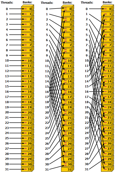
Different memory access patterns and their performance impact (Source: NVIDIA CUDA Programming Guide)

When NOT to Use: Standard Transformer models (text-based) don’t benefit from texture memory since they process 1D sequences without spatial structure.

Unified Memory: Bridging CPU and GPU

What is Unified Memory? Unified Memory allows both CPU and GPU to access the same memory address space, simplifying programming but with performance trade-offs.

Characteristics:

• Access Time: Variable (includes potential PCIe transfer overhead)
• Energy Consumption: High (due to CPU-GPU transfers)
• Capacity: Can exceed GPU memory (uses system RAM)
• Bandwidth: Limited by PCIe (32 GB/s PCIe 4.0 x16)

How It Works: The CUDA runtime automatically migrates data between CPU and GPU memory on-demand:

# Unified Memory allocation
data = torch.randn(10000, 10000).pin_memory()  # CPU memory
data = data.cuda()  # Migrates to GPU when accessed

# Automatic migration happens transparently
result = model(data)  # Data moved to GPU if needed

Use Cases:

• Models larger than GPU memory
• CPU-GPU collaborative algorithms
• Prototyping and debugging

Performance Trade-offs:

Advantages:

• Simpler programming model
• Handles out-of-memory scenarios gracefully
• Useful for sparse data structures

Disadvantages:

• Page faults cause significant overhead
• PCIe bandwidth is 50× lower than HBM bandwidth
• Unpredictable performance

Example Scenario: Training a 100B parameter model on a 40GB A100:

• Parameters: 400 GB (FP32)
• Options: Model parallelism OR Unified Memory with CPU offloading
• Unified Memory allows training but with 10-50× slowdown for offloaded portions

Best Practice: Use Unified Memory for convenience during development, but optimize for explicit memory management in production.

Complete Memory Hierarchy Comparison

Memory Type	Access Time	Energy	Capacity (A100)	Bandwidth	Scope	Usage Pattern
Registers	1-2 cycles	Lowest	~64 KB/SM	N/A	Thread-private	Scalar values, loop counters
Shared Memory	4-8 cycles	Low	100 KB/SM	~20 TB/s	Thread block	Explicitly managed tiles
L2 Cache	30-50 cycles	Moderate	6 MB	~4 TB/s	GPU-wide	Automatic caching
Global Memory (HBM)	200-400 cycles	High	40/80 GB	1555 GB/s	GPU-wide	Model weights, activations
Texture Memory	200-400 cycles	Moderate	Part of HBM	1555 GB/s	GPU-wide	2D spatial data
Unified Memory	Variable	Highest	System RAM	32 GB/s (PCIe)	CPU+GPU	Oversubscription, prototyping

Key Insights:

Speed vs Capacity Trade-off:

• Fastest memory (registers): Smallest capacity (~64 KB)
• Largest memory (HBM): Slowest access time (200-400 cycles)
• This is a fundamental hardware constraint

Energy Efficiency: Moving data from HBM costs ~100× more energy than accessing shared memory. Algorithms that minimize data movement are critical for energy-efficient AI.

Bandwidth Hierarchy:

Shared Memory (20 TB/s) > L2 Cache (4 TB/s) > HBM (1.5 TB/s) > PCIe (32 GB/s)

Memory Hierarchy in Action: Transformer Example

Let’s trace how different memory types are used during a single attention computation:

Step 1: Load Model Weights

W_Q, W_K, W_V = load_weights_from_hbm()

Memory: Global Memory → 200-400 cycles per weight

Step 2: Compute Q, K, V Projections

Q = matmul(input, W_Q)

Optimization:

• Load tiles of W_Q into Shared Memory
• Each thread block processes a tile
• Intermediate results stored in Registers

Step 3: Compute Attention Scores \(\text{scores} = \frac{QK^T}{\sqrt{d_k}}\)

Memory Flow:

1. Load Q tile into Shared Memory (4-8 cycles)
2. Load K tile into Shared Memory (4-8 cycles)
3. Compute dot products using Registers (1-2 cycles per op)
4. Store results back to Global Memory (200-400 cycles)

Step 4: Apply Softmax

attention_weights = softmax(scores)

Cache Behavior: If scores recently written, likely in L2 Cache (30-50 cycles) - avoids full global memory round-trip.

Total Memory Hierarchy Usage:

• Registers: ~90% of arithmetic operations
• Shared Memory: Tile loading for matrix multiplications
• L2 Cache: Frequently reused intermediate results
• Global Memory: Input/output and weight storage

Key Takeaways

Global Memory Characteristics: Slow per-access (200-400 cycles) but massive bandwidth (1555 GB/s). Optimization focuses on batching operations and coalescing accesses.

HBM Technology: 3D-stacked memory providing 3× higher bandwidth than GDDR6, essential for large model training where billions of parameters must move efficiently.

Specialized Memory: Texture memory accelerates 2D spatial data access for vision models; Unified Memory simplifies CPU-GPU collaboration but with 50× bandwidth penalty.

The Hierarchy in Practice: Real applications use all memory types simultaneously - registers for computation, shared memory for tiling, L2 for automatic caching, and global memory for bulk storage.

Energy Considerations: Data movement from HBM costs 100× more energy than accessing shared memory. Memory-efficient algorithms are also energy-efficient algorithms.

What’s Next?

In Part 3, we’ll explore practical optimization techniques, memory bandwidth bottlenecks, the roofline model, and tools for measuring memory performance.

---

Series Navigation:

• Part 1: Understanding the Hierarchy
• Part 2: Global and Specialized Memory (Current)
• Part 3: Optimization and Best Practices

References:

• MIT 6.5940: TinyML and Efficient Deep Learning Computing (Fall 2024)
• NVIDIA A100 GPU Architecture Whitepaper
• CUDA C++ Programming Guide: Memory Hierarchy
• Understanding the A100 GPU Memory Subsystem