Efficiency Metrics Part 3: Computation Metrics (MACs and FLOPs)

In the previous parts, we covered performance and memory metrics. Now we tackle computation metrics—the numbers that tell us how much actual work a neural network performs. These metrics are hardware-agnostic and reveal the fundamental computational complexity of your model.

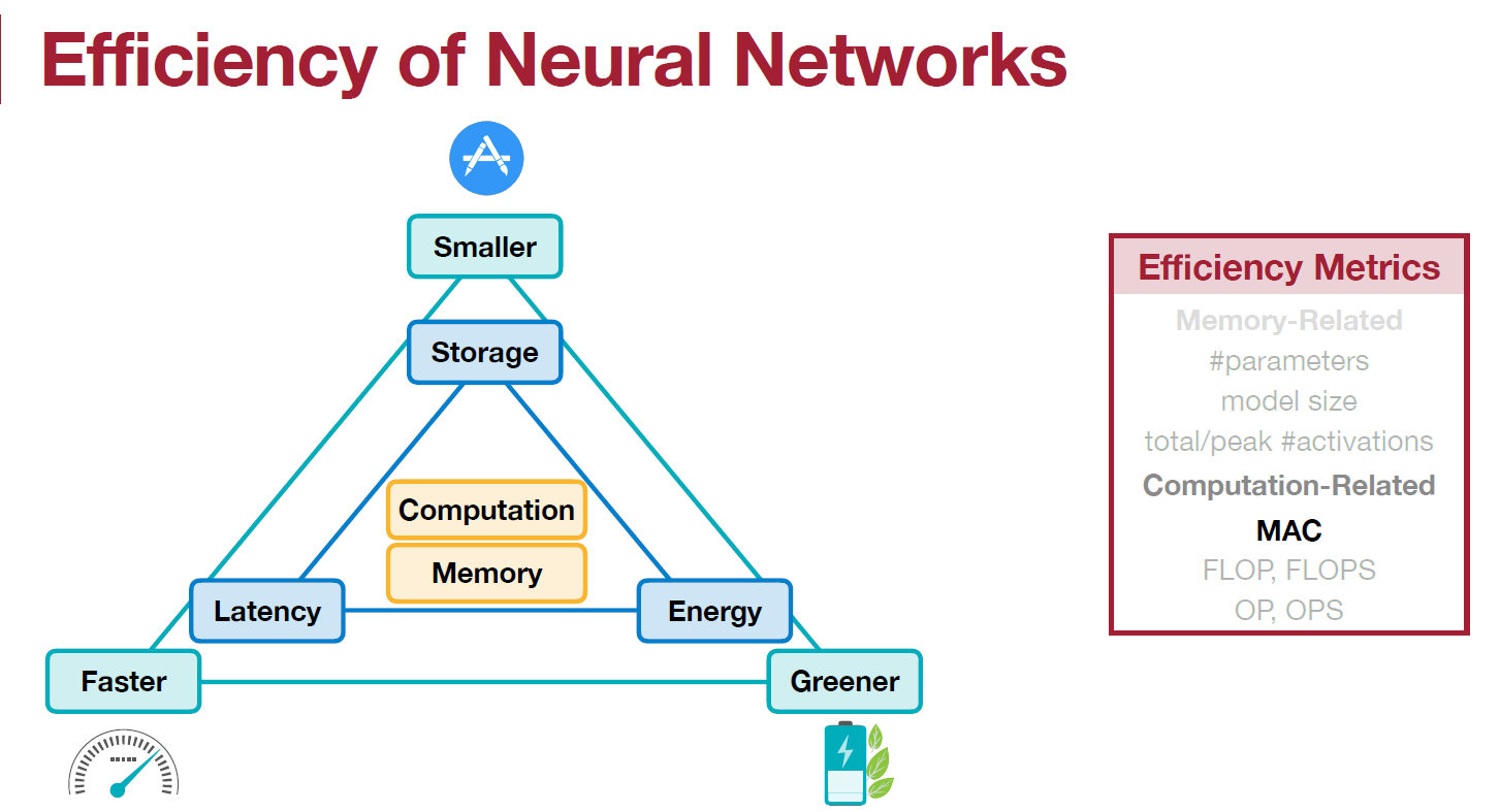
Computation metrics in the efficiency framework (Source: MIT 6.5940 Lecture 2)

Understanding MACs: The Building Block

MACs = Multiply-Accumulate Operations

A MAC is the most fundamental operation in neural networks:

\[\text{result} = \text{result} + (a \times b)\]

One MAC performs:

1. A multiplication ($a \times b$)
2. An addition to accumulate the result

Why MACs Matter

Neural networks are essentially massive sequences of MACs:

• Matrix multiplication: Every dense layer
• Convolutions: Sliding windows of MACs
• Attention mechanisms: Weighted combinations using MACs

All the magic in deep learning—from image recognition to language understanding—boils down to performing millions or billions of these simple operations.

Calculating MACs for Matrix Operations

Matrix-Vector Multiplication

For a matrix of size $m \times n$ multiplied by a vector of size $n \times 1$:

\[\text{MACs} = m \times n\]

Example:

Matrix: 1000 × 512
Vector: 512 × 1
Output: 1000 × 1

MACs = 1000 × 512 = 512,000 MACs

Matrix-Matrix Multiplication (GEMM)

For matrix $A$ of size $m \times k$ multiplied by matrix $B$ of size $k \times n$:

\[\text{MACs} = m \times n \times k\]

Example:

A: 1000 × 512
B: 512 × 256
Output C: 1000 × 256

MACs = 1000 × 256 × 512 = 131 million MACs

Each element in the output matrix requires $k$ MACs (one per element in the dot product).

MACs by Layer Type

Different neural network layers have different MAC formulas. Here’s a comprehensive reference:

Layer Type	MAC Formula	Intuition
Linear	$C_o \times C_i$	Every output needs all inputs
Convolution	$C_o \times C_i \times k_h \times k_w \times h_o \times w_o$	Kernel applied at each output position
Grouped Conv	$\frac{C_o}{g} \times \frac{C_i}{g} \times k_h \times k_w \times h_o \times w_o \times g$	Divided across groups
Depthwise Conv	$C_o \times k_h \times k_w \times h_o \times w_o$	No cross-channel computation

Where:

• $C_i$, $C_o$: Input and output channels
• $k_h$, $k_w$: Kernel height and width
• $h_o$, $w_o$: Output feature map height and width
• $g$: Number of groups

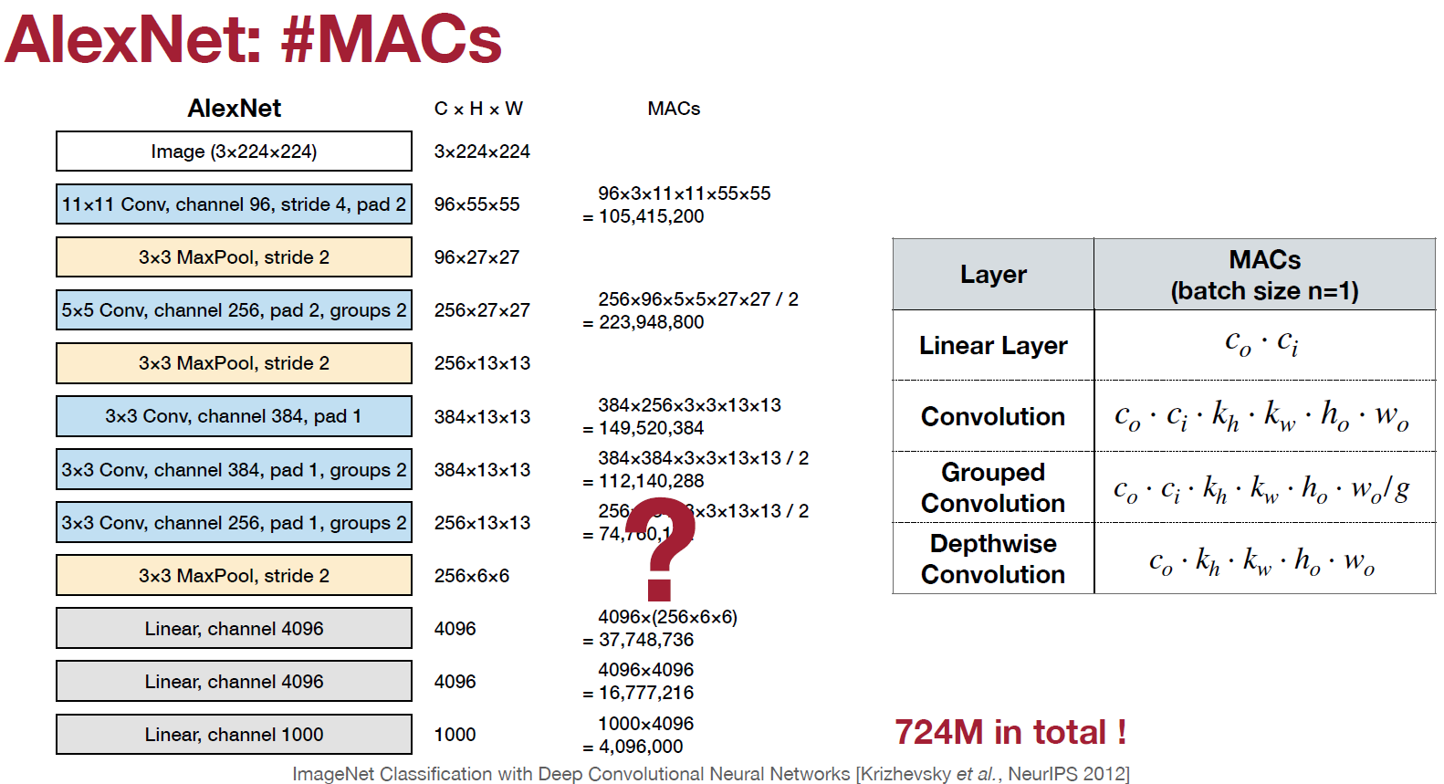
Visual representation of MAC operations in matrix multiplication (Source: MIT 6.5940 Lecture 2)

Concrete Example: Standard Convolution

Input: 224×224×3 (RGB image)
Kernel: 3×3, 64 filters
Output: 224×224×64

MACs = C_o × C_i × k_h × k_w × h_o × w_o
     = 64 × 3 × 3 × 3 × 224 × 224
     = 87,096,000 MACs
     ≈ 87 million MACs

Optimization Strategy: Depthwise Separable Convolutions

One powerful technique for reducing computation is depthwise separable convolutions, which split a standard convolution into two steps:

Standard Convolution:

Input: 224×224×32
Output: 224×224×64
Kernel: 3×3

MACs = 64 × 32 × 3 × 3 × 224 × 224
     = 2.97 billion MACs

Depthwise Separable Convolution:

Step 1 - Depthwise (3×3 per channel):

MACs = 32 × 3 × 3 × 224 × 224
     = 145.4 million

Step 2 - Pointwise (1×1 cross-channel):

MACs = 64 × 32 × 1 × 1 × 224 × 224
     = 1.03 billion

Total: 145.4M + 1.03B = 1.18 billion MACs

Reduction: 2.97B → 1.18B = 60% fewer MACs!

This technique is fundamental to efficient architectures like MobileNet and EfficientNet.

FLOPs: Floating Point Operations

FLOPs = Floating Point Operations (plural)

While MACs measure multiply-accumulate pairs, FLOPs count individual floating-point operations.

Key Distinction

Don’t confuse:

• FLOPs (plural): Number of operations—what we measure for models
• FLOPS (with capital S): Operations per second—hardware throughput capability

Relationship to MACs

One MAC consists of two floating-point operations:

\[\text{FLOPs} = 2 \times \text{MACs}\]

1. One FLOP for the multiplication
2. One FLOP for the addition

Example: AlexNet

AlexNet MACs: 724 million

FLOPs = 2 × 724M = 1.448 billion FLOPs
      ≈ 1.4 GFLOPs (GigaFLOPs)

Common Units and Model Scale

Unit	Operations	Typical Model
KFLOPs	$10^3$	Tiny embedded models
MFLOPs	$10^6$	Mobile models (MobileNet)
GFLOPs	$10^9$	Desktop models (ResNet-50)
TFLOPs	$10^{12}$	Large language models
PFLOPs	$10^{15}$	Training GPT-scale models

Model Complexity Comparison

Model	FLOPs	Relative Cost
MobileNetV2	0.3 G	1× (baseline)
SqueezeNet	0.8 G	2.7×
ResNet-50	4.1 G	13.7×
ResNet-152	11.5 G	38.3×
VGG-16	15.5 G	51.7×

VGG-16 requires over 50× more computation than MobileNetV2, yet often achieves similar accuracy!

From FLOPs to Real-World Performance

Hardware Throughput (FLOPS)

Different hardware has vastly different compute capabilities:

Hardware	Peak FLOPS (FP32)	Typical Cost
iPhone 12 CPU	~100 GFLOPS	-
NVIDIA RTX 3090	35.6 TFLOPS	$1,500
NVIDIA A100	19.5 TFLOPS	$10,000
TPU v4	275 TFLOPS	Cloud only

Theoretical Inference Time

The theoretical minimum time to run a model:

\[\text{Time} = \frac{\text{Model FLOPs}}{\text{Hardware FLOPS}}\]

Example:

Model: ResNet-50 (4.1 GFLOPs)
Hardware: NVIDIA RTX 3090 (35.6 TFLOPS = 35,600 GFLOPS)

Theoretical time = 4.1 / 35,600 
                 = 0.000115 seconds
                 = 0.115 milliseconds

Actual measured time: ~5 ms

Efficiency: 0.115 / 5 = 2.3%

Only 2.3% of theoretical peak performance! Why?

The Reality Gap

FLOPs are a theoretical measure. Real-world performance suffers from:

1. Memory bandwidth bottlenecks: Data can’t reach the compute units fast enough
2. Data transfer overhead: Moving tensors between CPU and GPU
3. Kernel launch latency: GPU operations have startup costs
4. Non-optimal tensor shapes: Hardware works best with specific dimensions
5. Software inefficiencies: Framework overhead, compilation issues

Key Insight: Low FLOPs doesn’t guarantee fast inference. Memory access patterns and hardware utilization matter just as much.

Key Takeaways

MACs (Multiply-Accumulate Operations):

• Fundamental unit of neural network computation
• Formula varies by layer type (linear, convolution, grouped, depthwise)
• Depthwise separable convolutions can reduce MACs by 60%+ while maintaining accuracy

FLOPs (Floating Point Operations):

• FLOPs = 2 × MACs (one multiply + one add)
• Hardware-agnostic measure of computational complexity
• Ranges from MFLOPs (mobile) to TFLOPs (LLMs) to PFLOPs (training)

Theoretical vs. Real Performance:

• Theoretical inference time = Model FLOPs ÷ Hardware FLOPS
• Actual performance often 10-100× slower due to memory bandwidth and overhead
• Optimization requires considering both computation AND memory access patterns

Optimization Strategy Table:

Goal	Primary Techniques	Metrics Improved
Reduce computation	Depthwise separable convs, NAS	FLOPs, MACs
Reduce latency	Quantization, pruning, distillation	Latency, FLOPs
Increase throughput	Larger batches, hardware acceleration	Throughput, FLOPS

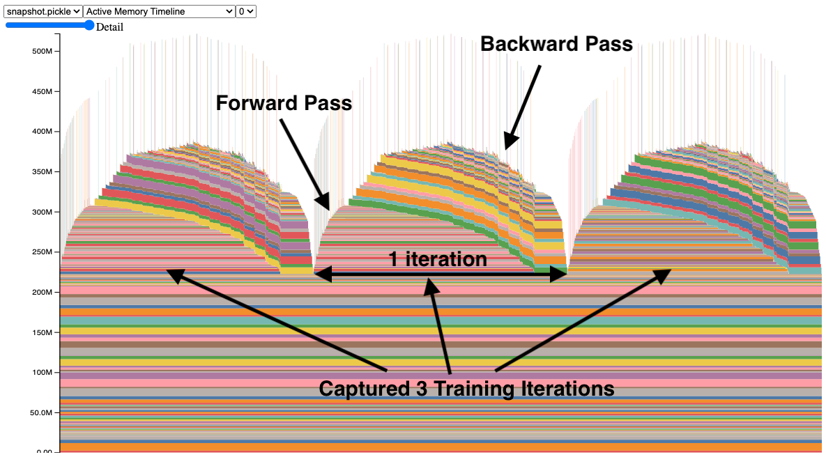
Memory and computation visualization over time (Source: PyTorch Blog)

What’s Next?

Now that you understand all three efficiency metric categories (performance, memory, and computation), you can:

Profile Your Models: Use tools like torchprofile or thop to measure MACs/FLOPs in your architectures

Compare Architectures: Make informed decisions—a model with 10× fewer FLOPs might be worth slight accuracy loss

Optimize Effectively: Target the right metrics for your use case (latency vs. throughput vs. memory)

Deploy with Confidence: Predict whether your model will fit and run efficiently on target hardware

In future posts, we’ll explore specific optimization techniques like quantization, pruning, and knowledge distillation—armed with the metrics to measure their impact!

---

Series Navigation:

• Part 1: Performance Metrics
• Part 2: Memory Metrics
• Part 3: Computation Metrics (Current)

References:

• MIT 6.5940: TinyML and Efficient Deep Learning (Fall 2024) - Lecture 2: Basics - Primary source for this content
• Han, Song, et al. “Deep Compression: Compressing Deep Neural Networks with Pruning, Trained Quantization and Huffman Coding.” ICLR 2016.
• Howard, Andrew G., et al. “MobileNets: Efficient Convolutional Neural Networks for Mobile Vision Applications.” arXiv:1704.04861 (2017).
• Sandler, Mark, et al. “MobileNetV2: Inverted Residuals and Linear Bottlenecks.” CVPR 2018.