Neural Network Pruning Part 5: Lottery Ticket Hypothesis and Training Sparse Networks

Rethinking How We Train Pruned Networks

In Part 4, we mastered the practical art of pruning:

• Layer-wise pruning ratios for optimal compression
• Iterative pruning with fine-tuning for minimal accuracy loss
• AutoML (AMC) for automated pruning decisions
• Combining pruning with quantization for extreme efficiency

But throughout, we followed a standard paradigm:

1. Train a dense network to convergence
2. Prune unnecessary weights
3. Fine-tune to recover accuracy

This raises fundamental questions:

• Why do we need dense networks for training?
• Do sparse subnetworks exist that could have been trained directly?
• Can we train sparse from scratch and save all that wasted computation?

This part explores groundbreaking research that challenges conventional wisdom about pruning and reveals surprising truths about neural network training.

The Lottery Ticket Hypothesis: A Paradigm Shift

The Core Question

Traditional belief: Dense networks are necessary for training. Pruning removes redundant weights after training.

Lottery Ticket Hypothesis asks: What if the dense network contains a sparse subnetwork (“winning lottery ticket”) that could have been trained in isolation to match the original’s performance?

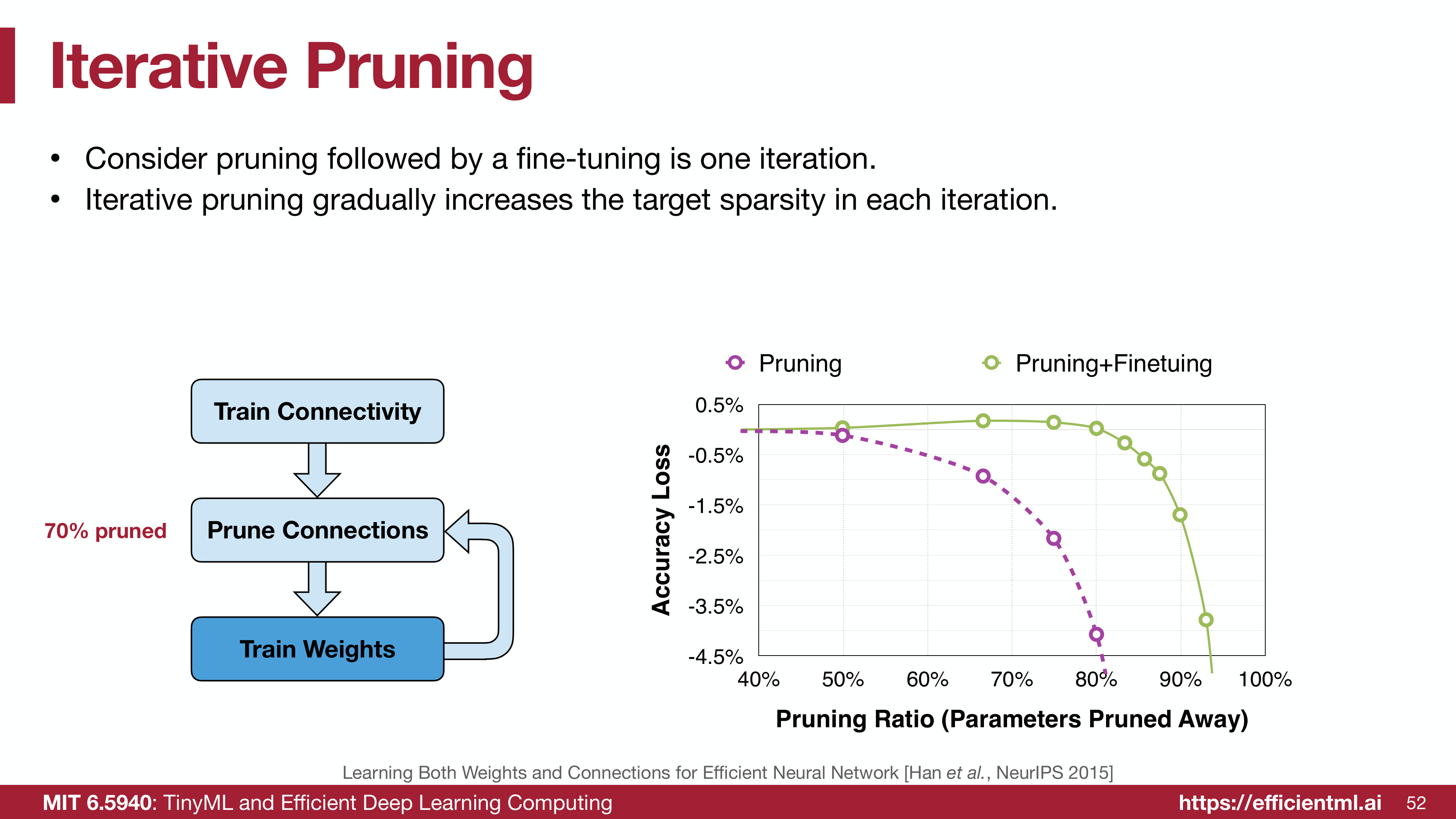
The Lottery Ticket Hypothesis: sparse subnetworks exist that match dense performance

The Hypothesis Statement

Lottery Ticket Hypothesis (Frankle & Carbin, 2019):

A randomly-initialized, dense neural network contains a subnetwork that is initialized such that—when trained in isolation—it can match the test accuracy of the original network after training for at most the same number of iterations.

Translation: Hidden inside every large network is a smaller “winning ticket” that, if we could find it and train it from scratch, would work just as well.

Why “Lottery Ticket”?

Analogy: Training a neural network is like buying many lottery tickets:

• Dense network = buying 1000 tickets
• Most tickets lose (most weights aren’t crucial)
• A few tickets win (sparse subnetwork with good initialization)
• Winning requires both the right structure AND the right initialization

Key insight: It’s not just about which weights to keep, but also their initial values.

Finding Winning Lottery Tickets

The Iterative Magnitude Pruning (IMP) Algorithm

Step-by-step process:

# 1. Randomly initialize the network
model = create_network()
initial_weights = save_weights(model)  # θ₀

# 2. Train to convergence
train(model, epochs=100)
trained_weights = save_weights(model)  # θ_trained

# 3. Identify weights to prune (e.g., smallest 20%)
mask = create_mask_from_magnitude(trained_weights, pruning_rate=0.20)

# 4. Reset remaining weights to their INITIAL values
model = load_weights(model, initial_weights * mask)

# 5. Train the sparse network from scratch
train(model, epochs=100)

# 6. Compare performance with original dense network

Critical detail: We don’t use the trained weights—we reset to initial values with the pruning mask!

Iterative Application

To find tickets at higher sparsity levels, repeat the process:

# Start with dense network
sparsity = 0.0
mask = ones_like(model.weights)

for iteration in range(15):  # Increase sparsity gradually
    # Train with current mask
    model = initialize_with_mask(initial_weights, mask)
    train(model, epochs=100)
    
    # Prune another 20%
    new_mask = prune_smallest_magnitude(model, rate=0.20)
    mask = mask * new_mask  # Compound pruning
    
    # Evaluate sparse subnetwork
    sparse_model = initialize_with_mask(initial_weights, mask)
    train(sparse_model, epochs=100)
    
    sparsity = 1 - mask.sum() / mask.numel()
    print(f"Sparsity: {sparsity:.1%}, Accuracy: {evaluate(sparse_model):.2%}")

Experimental Results

LeNet on MNIST:

• Dense network: 99.2% accuracy, 266K parameters
• Winning ticket (99% sparse): 99.1% accuracy, 3K parameters
• Random sparse (99%): 95.0% accuracy (fails to train!)

Key finding: With the right initialization, 1% of weights is enough!

ResNet-20 on CIFAR-10:

Sparsity	Dense Acc	Winning Ticket	Random Sparse
0%	91.2%	-	-
50%	91.2%	91.0%	87.5%
80%	91.2%	90.5%	72.1%
95%	91.2%	89.2%	Random fails

Observation: Winning tickets maintain performance, random sparse networks collapse.

Understanding Why Lottery Tickets Work

The Role of Initialization

Why does initial weight matter so much?

1. Loss Landscape Navigation:
   • Good initialization starts near a favorable basin
   • Training proceeds along a beneficial trajectory
   • Sparse network reaches good minimum
2. Information Preservation:
   • Initial weights encode “lottery ticket information”
   • Pruning mask selects weights aligned with useful gradients
   • Together they form a trainable configuration
3. Gradient Flow:
   • Good initial weights have appropriate scale
   • Enable effective gradient propagation
   • Critical for deep networks

Warm-up: The Learning Rate Rewinding Trick

Problem: At higher sparsity (>95%), even winning tickets struggle to train from iteration 0.

Solution: Learning Rate Rewinding (Frankle et al., 2020)

Instead of resetting to initialization (iteration 0), reset to weights from early training (iteration k):

# Standard lottery ticket (fails at high sparsity)
model = initialize_with_mask(weights_at_iter_0, mask)
train(model, epochs=100)

# Learning rate rewinding (works at high sparsity!)
model = initialize_with_mask(weights_at_iter_k, mask)  # k = 500-5000 steps
train(model, epochs=100, lr_schedule_from_iter_k)

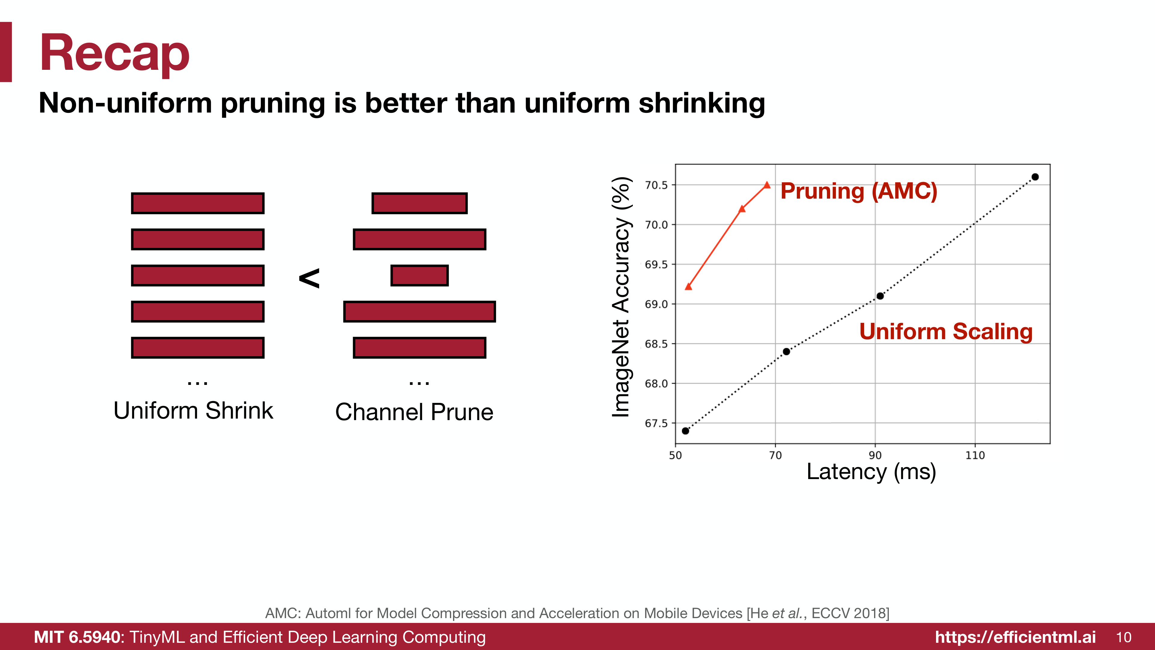
Different initialization strategies: iteration 0 vs. early training vs. late training

Why it works:

• Weights at iteration k have learned low-level features
• Still plastic enough to learn task-specific patterns
• Provides better starting point than random initialization

Results on ResNet-50 (ImageNet):

Rewind Point	Sparsity	Top-1 Accuracy
Iter 0	80%	68.2%
Iter 0	90%	Fails to converge
Iter 10K	80%	75.8%
Iter 10K	90%	74.1%
Iter 20K	80%	76.1%
Iter 20K	90%	75.3%

Sweet spot: Rewinding to 10-20K iterations (2-4% of total training).

Practical Implications of Lottery Tickets

What Lottery Tickets Tell Us

1. Overparameterization helps training, not just representation
   • Dense networks aren’t inherently better
   • They’re easier to train because they contain many potential solutions
   • Sparse networks CAN work if initialized correctly
2. Pruning is partly about finding good initializations
   • Traditional pruning: train → prune → fine-tune
   • Lottery tickets: train → prune → reset → retrain
   • Both work, but understand different aspects
3. Transfer learning implications
   • Winning tickets might transfer across tasks
   • Pre-trained sparse networks could be more efficient
   • Active research area

Limitations and Challenges

Computational cost:

• Finding tickets requires training to convergence multiple times
• Each pruning iteration = full training run
• 15 iterations × 100 epochs = 1500 epochs total
• More expensive than standard train-prune-fine-tune

Scalability:

• Works well for small networks (LeNet, ResNet-20)
• Challenging for very large networks (GPT, BERT)
• Requires significant compute resources

Practical deployment:

• Most practitioners still use standard pruning
• Lottery tickets are more for understanding than production
• Research tool rather than deployment strategy

Beyond Lottery Tickets: Modern Sparse Training

Dynamic Sparse Training (DST)

Problem: Lottery tickets require multiple full training cycles.

Solution: Train sparse from the start, with dynamic weight updates.

The Algorithm:

# Initialize sparse network (random mask)
mask = random_sparse_mask(sparsity=0.90)
model = initialize_network()
model.apply_mask(mask)

for epoch in range(100):
    # Standard training step
    loss = train_step(model)
    
    # Every N epochs: update the mask
    if epoch % UPDATE_FREQUENCY == 0:
        # Drop connections with smallest magnitude
        drop_mask = get_smallest_weights(model, drop_fraction=0.20)
        
        # Grow new connections (random or gradient-based)
        grow_mask = select_new_connections(model, grow_fraction=0.20)
        
        # Update mask: drop old, add new
        mask = (mask - drop_mask) + grow_mask
        model.apply_mask(mask)

Key idea: The sparse structure evolves during training, not fixed after pruning.

Methods for growing connections:

1. Random: Add random new connections
2. Gradient-based: Add connections with largest gradients
3. Momentum-based: Use gradient momentum to predict useful connections

Results (RigL method on ImageNet):

Method	Sparsity	Top-1 Acc	Training Cost
Dense baseline	0%	76.1%	100%
Lottery ticket	80%	75.8%	1500%
RigL (DST)	80%	75.6%	120%

Advantage: Near-identical accuracy with 10× lower training cost than lottery tickets!

Straight-Through Estimators (STE)

Problem: Binary masks (0 or 1) aren’t differentiable.

Solution: Use different functions for forward and backward passes.

Forward pass (discrete):

mask = (scores > threshold).float()  # Binary: 0 or 1
output = input * mask

Backward pass (continuous):

# Pretend mask is differentiable
grad_mask = grad_output * input  # Continuous gradient

Why it works:

• Forward pass: Exact sparse computation
• Backward pass: Smooth gradient flow
• Network learns which connections to keep/remove

Application in learned pruning:

# Learnable pruning scores
scores = nn.Parameter(torch.randn(num_weights))

# Forward: apply binary mask
mask = (scores > 0).float()  # STE here!
pruned_weights = weights * mask

# Backward: update scores based on gradients
scores.grad = compute_gradients(loss, scores)

Sparse Training from Scratch: Magnitude Pruning at Init

Question: Can we prune BEFORE training?

Idea: Some initializations are better than others for sparse training.

Methods:

1. SNIP (Single-shot Network Pruning):

• Compute connection sensitivity at initialization

• Sensitivity =

  ∂loss/∂weight

  at initialization

• Prune lowest sensitivity connections
• Train the resulting sparse network

2. GraSP (Gradient Signal Preservation):

• Prune connections that preserve gradient flow
• Maintain strong gradient magnitudes through layers
• Ensures trainability of pruned network

3. SynFlow (Synaptic Flow):

• Iteratively prune connections based on “synaptic saliency”

• Score =

  weight

  ×

  gradient of weight

• Layer-balanced pruning

Results on ResNet-50 (90% sparsity):

Method	Prune When?	Top-1 Acc	Training Time
Magnitude (post-train)	After training	75.2%	100% + fine-tune
Lottery ticket	After + retrain	75.8%	1500%
Random (at init)	Before training	68.1%	100%
SNIP (at init)	Before training	72.4%	100%
GraSP (at init)	Before training	73.6%	100%
SynFlow (at init)	Before training	74.1%	100%

Advantage: Pruning at initialization with smart methods gets 90-95% of post-training pruning quality with no extra training cost!

Hardware-Aware Sparse Training

The Deployment Gap

Problem: High sparsity doesn’t always mean fast inference.

Example:

Model: 90% sparse (10% weights remain)
Expected speedup: 10×
Actual speedup on GPU: 1.2×  😞

Why? Hardware doesn’t efficiently handle irregular sparsity patterns.

N:M Structured Sparsity

Solution: Train networks with hardware-friendly sparsity patterns.

N:M sparsity: Out of every M consecutive weights, keep exactly N non-zero.

Examples:

• 2:4 sparsity: 2 non-zero out of every 4 weights (50% sparse)
• 4:8 sparsity: 4 non-zero out of every 8 weights (50% sparse)

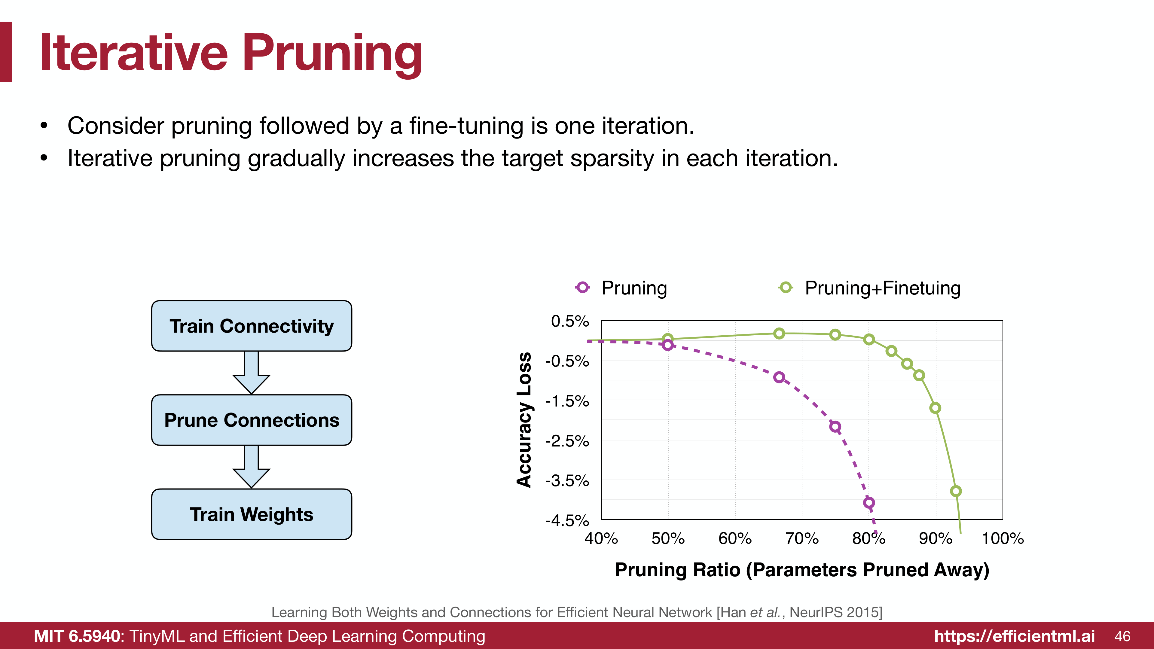
Structured sparse networks achieve real hardware speedup on modern GPUs

Training for N:M sparsity:

def apply_nm_sparsity(weight_tensor, n=2, m=4):
    # Reshape to groups of M weights
    shape = weight_tensor.shape
    reshaped = weight_tensor.reshape(-1, m)
    
    # For each group, keep top-N by magnitude
    topk_values, topk_indices = torch.topk(reshaped.abs(), n, dim=1)
    
    # Create mask
    mask = torch.zeros_like(reshaped)
    mask.scatter_(1, topk_indices, 1)
    
    # Apply mask and reshape back
    sparse_weight = (weight_tensor.reshape(-1, m) * mask).reshape(shape)
    return sparse_weight

# During training
for epoch in range(100):
    train_step(model)
    
    # Apply N:M sparsity constraint after each step
    for param in model.parameters():
        param.data = apply_nm_sparsity(param.data, n=2, m=4)

Hardware support:

• NVIDIA Ampere/Hopper GPUs: Native 2:4 sparsity support
• 2× speedup with 2:4 sparsity (compared to ~1.1× for unstructured)
• Minimal accuracy drop: 0.5-1% on most tasks

Results (BERT-base on SQuAD):

Method	Sparsity	F1 Score	GPU Speedup
Dense	0%	88.5	1.0×
Unstructured 50%	50%	88.1	1.1×
2:4 structured	50%	88.0	1.9×

Combining Sparse Training Techniques

The Optimal Pipeline

Based on current research, here’s a recommended approach:

Stage 1: Smart Initialization

# Use SynFlow or GraSP to find good initial mask
mask = synflow_pruning(model, target_sparsity=0.80)
model.apply_mask(mask)

Stage 2: Dynamic Sparse Training

# Train with mask updates (RigL-style)
for epoch in range(50):
    train_step(model)
    if epoch % 5 == 0:
        update_mask_dynamically(model, drop_rate=0.10, grow_rate=0.10)

Stage 3: Hardware-Aware Refinement

# Convert to N:M sparsity for deployment
for param in model.parameters():
    param.data = apply_nm_sparsity(param.data, n=2, m=4)

# Fine-tune with hardware-aware constraint
for epoch in range(10):
    train_step(model)
    enforce_nm_sparsity(model, n=2, m=4)

Stage 4: Quantization

# Combine with INT8 quantization
quantized_model = quantize(model, dtype=torch.qint8)

Final result:

• 50% sparse (2:4 pattern)
• 8-bit quantized
• ~8× compression from dense FP32
• ~2× inference speedup on Ampere GPU
• <1% accuracy drop

The Future: What’s Next for Sparse Neural Networks?

Emerging Research Directions

1. Sparse Large Language Models

• SparseGPT: Prune 50% of GPT-175B with minimal quality loss
• Mixture of Experts (MoE): Conditionally activate sparse subnetworks
• Adaptive computation: Different inputs use different sparsity levels

2. Sparse Vision Transformers

• Token pruning: Dynamically remove uninformative tokens
• Attention sparsity: Use sparse attention patterns
• Hierarchical pruning: Prune both tokens and model weights

3. Training-Free Pruning

• Prune based on architecture analysis alone
• No need for training data
• Useful for privacy-sensitive applications

4. Sparse Neural Architecture Search

• Search for both architecture AND sparsity pattern
• Co-optimize structure and density
• Find optimal sparse networks faster

Open Questions

1. Can we find lottery tickets in one shot?
   • Current methods require multiple training runs
   • Need faster winning ticket identification
2. Do lottery tickets transfer across tasks?
   • Can we find universal sparse initializations?
   • Would enable sparse pre-trained models
3. What’s the fundamental limit of sparsity?
   • How sparse can we go without losing capacity?
   • Are there task-dependent theoretical bounds?
4. How to make sparse training as efficient as sparse inference?
   • Current training still uses dense operations
   • Need hardware/software for sparse training acceleration

Practical Recommendations

For Researchers

Studying network pruning:

• Explore lottery tickets to understand trainability
• Use dynamic sparse training for compute-efficient experiments
• Consider hardware constraints early in design

Key papers to read:

1. The Lottery Ticket Hypothesis (Frankle & Carbin, 2019)
2. Stabilizing the Lottery Ticket Hypothesis (Frankle et al., 2020)
3. Rigging the Lottery: RigL (Evci et al., 2020)
4. SNIP, GraSP, SynFlow (various papers 2019-2020)

For Practitioners

Production deployment:

• Use traditional magnitude pruning + fine-tuning (most reliable)
• Consider 2:4 sparsity if using NVIDIA Ampere or newer
• Combine with quantization for maximum compression
• Always measure real hardware speedup, not just parameter count

Quick wins:

• Start with 50% unstructured pruning (safe, significant size reduction)
• Use iterative pruning with 5-10 rounds
• Fine-tune for 10% of original training epochs
• Validate accuracy on full test set

For Hardware Designers

Supporting sparsity:

• Implement N:M sparsity patterns (like NVIDIA’s 2:4)
• Provide software libraries for sparse operations
• Co-design sparsity patterns with ML researchers
• Consider variable sparsity levels (not just 50%)

Key Takeaways

1. Lottery Ticket Hypothesis shows sparse networks CAN train from scratch if initialized correctly

2. Initialization matters as much as structure for sparse network training

3. Learning rate rewinding extends lottery tickets to higher sparsity levels

4. Dynamic sparse training (RigL, SET, etc.) trains sparse networks efficiently without finding tickets

5. Pruning at initialization (SNIP, GraSP, SynFlow) can achieve competitive results with zero extra training cost

6. Hardware-aware sparsity patterns (2:4) deliver real speedups on modern GPUs

7. Combining techniques (sparse training + quantization) achieves best compression and speed

8. Production use cases should prioritize reliability over cutting-edge research methods

Conclusion: A New Era of Efficient Training

The lottery ticket hypothesis and modern sparse training methods represent a paradigm shift in how we think about neural network efficiency:

Old paradigm:

• Train large → Prune → Fine-tune
• Efficiency comes after training
• Sparsity is a post-processing step

New paradigm:

• Efficiency-aware from initialization
• Sparse training is competitive with dense
• Structure and initialization co-matter

The future is sparse:

• Models will be trained sparse from the start
• Hardware will natively support structured sparsity
• Sparse pre-trained models will become standard
• Training cost will decrease alongside inference cost

The tools and understanding now exist to train efficient sparse networks. The next frontier is making sparse training as ubiquitous and easy as dense training is today.

Thank you for following this series! From the energy crisis of massive models to the cutting edge of sparse neural networks, we’ve covered the complete landscape of neural network pruning. We hope these insights help you build more efficient AI systems.

---

Series Navigation:

• Part 1: Why Pruning Matters
• Part 2: Pruning Granularities
• Part 3: Pruning Criteria
• Part 4: Advanced Techniques
• Part 5: Lottery Tickets and Beyond (Current)

References:

• MIT 6.5940: TinyML and Efficient Deep Learning (Fall 2024)
• The Lottery Ticket Hypothesis (Frankle & Carbin, ICLR 2019)
• Stabilizing the Lottery Ticket Hypothesis (Frankle et al., 2020)
• Rigging the Lottery: Making All Tickets Winners (RigL, Evci et al., 2020)
• SNIP: Single-shot Network Pruning (Lee et al., ICLR 2019)
• GraSP: Pruning at Initialization (Wang et al., NeurIPS 2020)
• SynFlow: Towards Dense-to-Sparse Training (Tanaka et al., NeurIPS 2020)
• Accelerating Sparse Deep Neural Networks (Mishra et al., 2021)

Acknowledgments:

This comprehensive blog series on Neural Network Pruning is based on MIT 6.5940: TinyML and Efficient Deep Learning (Fall 2024) taught by Professor Song Han and his team at MIT Han Lab.

Special Thanks:

• Professor Song Han and the MIT Han Lab for pioneering efficient deep learning research
• The EfficientML.ai community for advancing the field of model compression
• All researchers cited whose groundbreaking work made this series possible
• The open-source community for tools like PyTorch, TensorFlow, and specialized pruning libraries

The insights, techniques, and case studies presented throughout this series draw heavily from cutting-edge research and practical implementations by these incredible teams. Their work is democratizing AI by making powerful models accessible on edge devices and reducing the environmental impact of deep learning.

For deeper exploration, we highly recommend taking the full MIT course and exploring the papers referenced throughout this series.