Neural Network Pruning Part 2: Pruning Granularities

Recap: Why Granularity Matters

In Part 1, we learned that pruning can reduce model size by 3-12× without losing accuracy. But there’s a catch: not all pruning patterns are created equal.

Imagine you’re reorganizing a bookshelf:

• Option 1: Remove random pages from random books (unstructured)
• Option 2: Remove entire books (structured)

Which is easier to manage? Obviously Option 2! Similarly, pruning granularity determines how we remove parameters from neural networks, affecting both compression ratio and hardware efficiency.

What is Pruning Granularity?

Pruning granularity refers to the unit at which we remove parameters from a neural network.

Think of it like demolishing parts of a building:

• Fine-grained: Remove individual bricks (maximum flexibility, hard to plan)
• Coarse-grained: Remove entire walls or rooms (less flexible, easy to plan)

The Fundamental Trade-off

There’s always a tension between two goals:

Goal	Favors	Trade-off
Maximum Compression	Fine-grained pruning	Harder to accelerate
Hardware Efficiency	Coarse-grained pruning	Lower compression ratio

Let’s explore this spectrum from fine to coarse granularity.

Fine-Grained (Unstructured) Pruning

What is It?

Fine-grained pruning removes individual weights from the network without any pattern or structure.

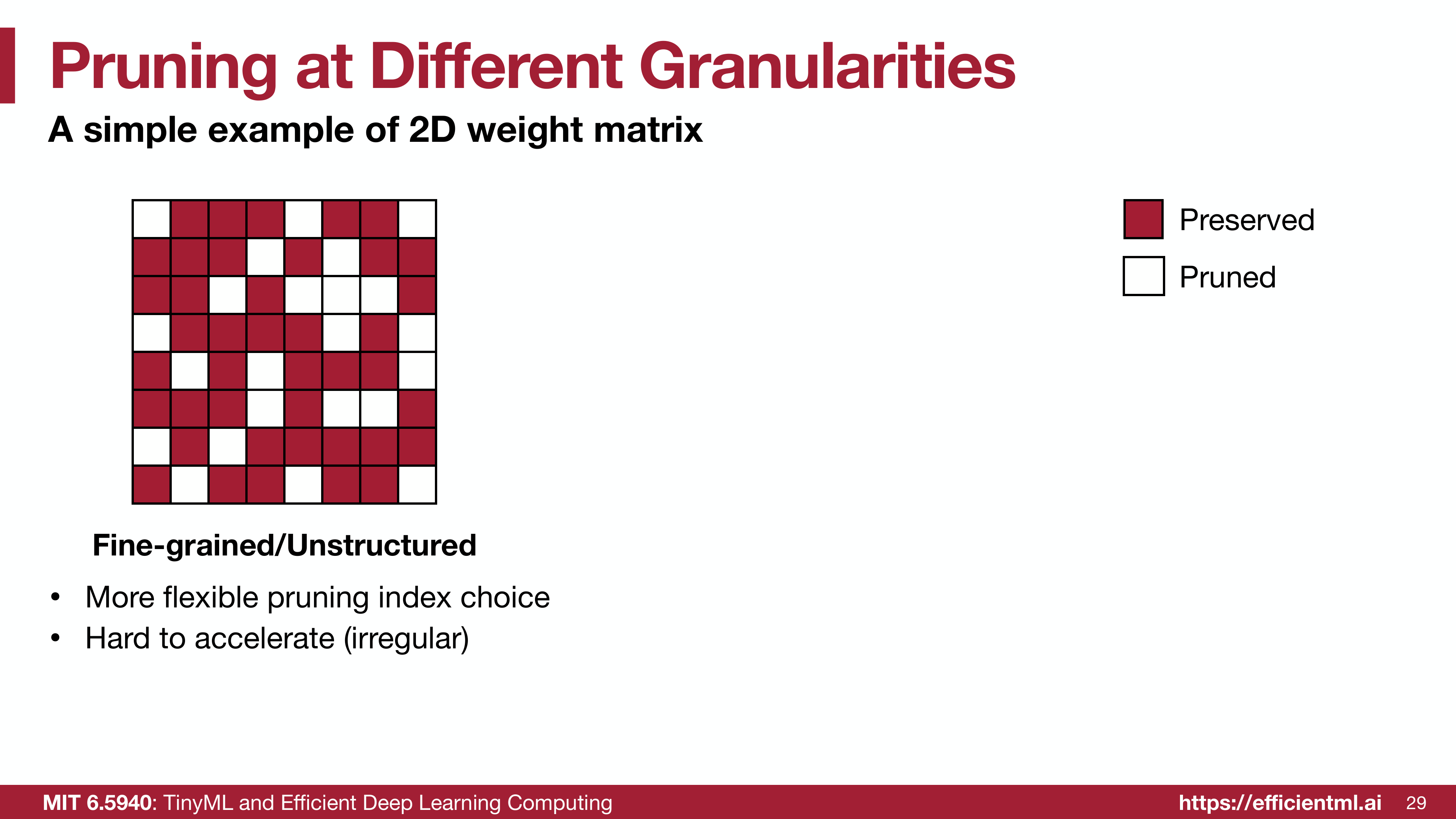
Fine-grained pruning: Individual weights are removed irregularly

Analogy: Like picking individual grapes from a bunch—you can choose exactly which ones to remove, but the remaining structure becomes irregular.

How It Works

For a simple weight matrix:

\[W = \begin{bmatrix} 0.8 & 0.1 & 0.9 & 0.05 \\ 0.3 & 0.7 & 0.2 & 0.6 \\ 0.1 & 0.4 & 0.85 & 0.15 \end{bmatrix}\]

After pruning small weights (e.g., < 0.3):

\[W_{\text{pruned}} = \begin{bmatrix} 0.8 & 0 & 0.9 & 0 \\ 0.3 & 0.7 & 0 & 0.6 \\ 0 & 0.4 & 0.85 & 0 \end{bmatrix}\]

Notice how zeros appear irregularly throughout the matrix.

Pros and Cons

Advantages: Maximum flexibility in choosing which weights to prune
Highest compression ratios (9-12× for AlexNet, VGG-16)
Can capture subtle patterns of weight importance

Disadvantages: Irregular memory access patterns slow down computation
No speedup on standard GPUs without special sparse libraries
Requires custom hardware (like EIE accelerator) for real speedup
Overhead from storing sparse indices

Where It Shines

Fine-grained pruning works best when:

• You need maximum compression (e.g., deploying on memory-constrained devices)
• You have specialized hardware that supports sparse operations
• Model size matters more than inference speed

Pattern-Based Pruning: The Middle Ground

What is N:M Sparsity?

Pattern-based pruning enforces a regular sparsity pattern where in every $M$ consecutive elements, exactly $N$ are pruned (set to zero).

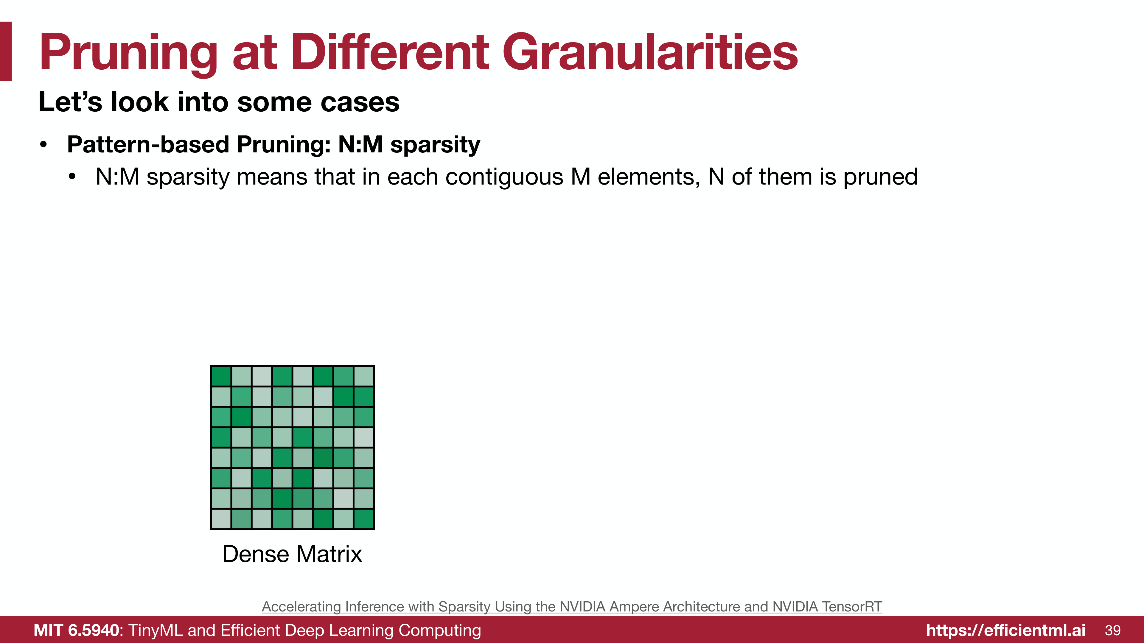
Original dense matrix before pruning

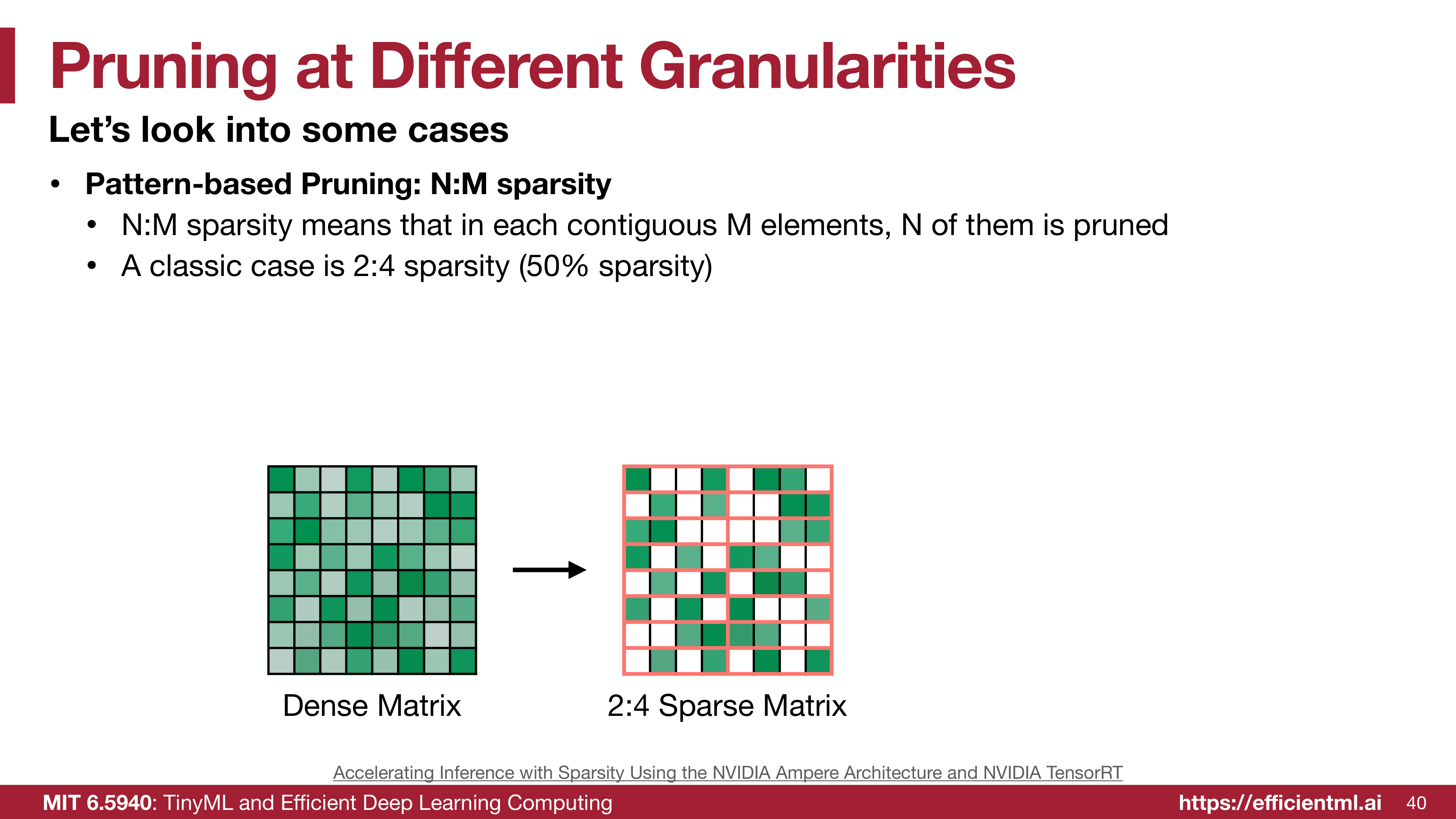
2:4 sparse matrix: exactly 2 out of every 4 elements are pruned

The 2:4 Sparsity Pattern (Most Common):

• In every group of 4 consecutive weights, exactly 2 are zero
• Results in 50% sparsity
• Supported by NVIDIA A100 GPU and newer architectures

How 2:4 Sparsity Works

Let’s see a concrete example:

Original weights:

[0.8, 0.3, 0.9, 0.1] | [0.5, 0.7, 0.2, 0.6]

After 2:4 pruning (keep 2 largest in each group of 4):

[0.8, 0.0, 0.9, 0.0] | [0.0, 0.7, 0.0, 0.6]

Compressed format:

• Non-zero values: [0.8, 0.9, 0.7, 0.6]
• 2-bit indices: [00, 10, 01, 11] (indicating positions 0,2 and 1,3)

Pros and Cons

Advantages: Hardware acceleration on NVIDIA Ampere GPUs (~2× speedup)
Predictable memory access patterns
Good compression (50% sparsity guaranteed)
Maintains accuracy on most tasks
Easy to implement with simple masking

Disadvantages: Less flexible than fine-grained pruning
Fixed 50% sparsity (can’t go higher without custom patterns)
Requires retraining to adapt to the constraint

Real-World Performance

NVIDIA Reports (2020):

• Theoretical speedup: 2×
• Measured BERT inference speedup: ~1.5×
• Accuracy retention: >99% on most NLP benchmarks

Coarse-Grained (Structured) Pruning

What is It?

Structured pruning removes entire organized groups of parameters:

• Channels (filters in convolutional layers)
• Neurons (entire rows/columns in matrices)
• Layers (in extreme cases)

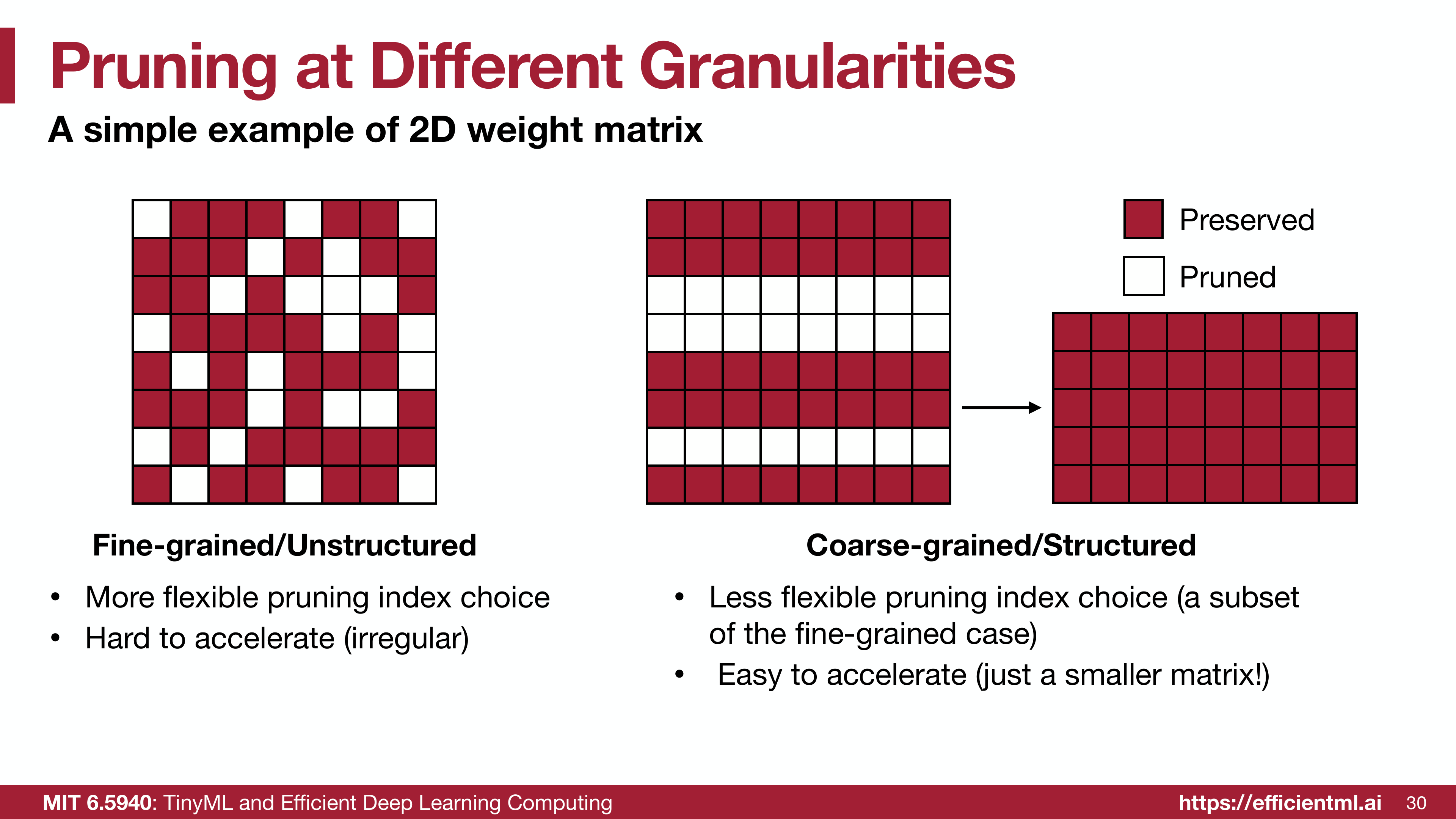
Coarse-grained pruning: Entire rows or columns are removed

Analogy: Like removing entire shelves from a bookcase—you can’t pick individual books, but the remaining structure is clean and organized.

Understanding Convolutional Layer Pruning

Convolutional layers have 4 dimensions:

\[W \in \mathbb{R}^{C_{\text{out}} \times C_{\text{in}} \times K_h \times K_w}\]

Where:

• $C_{\text{out}}$: Number of output channels (filters)
• $C_{\text{in}}$: Number of input channels
• $K_h, K_w$: Kernel height and width

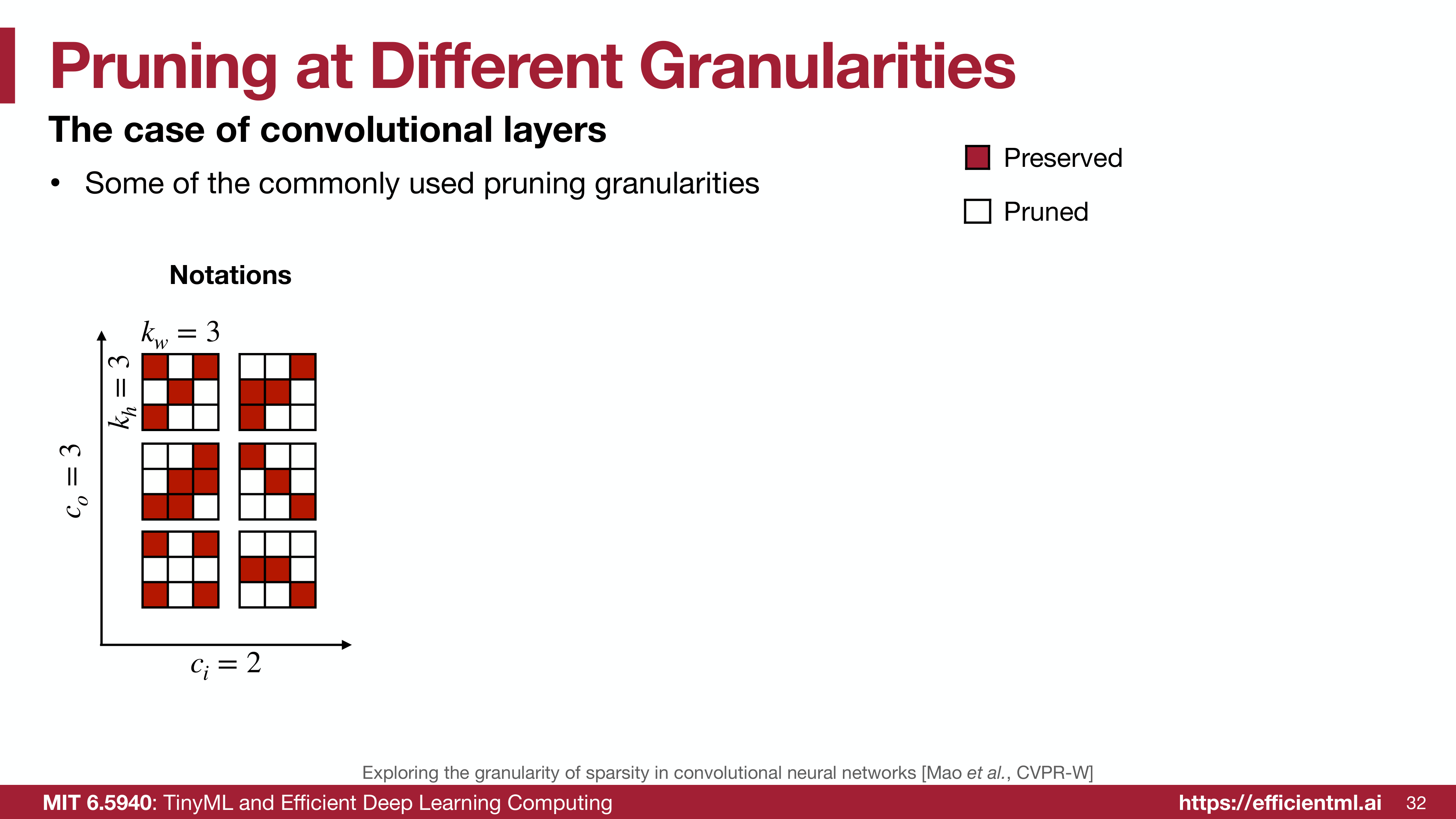
Four dimensions of convolutional weights provide multiple pruning options

This gives us multiple granularity choices:

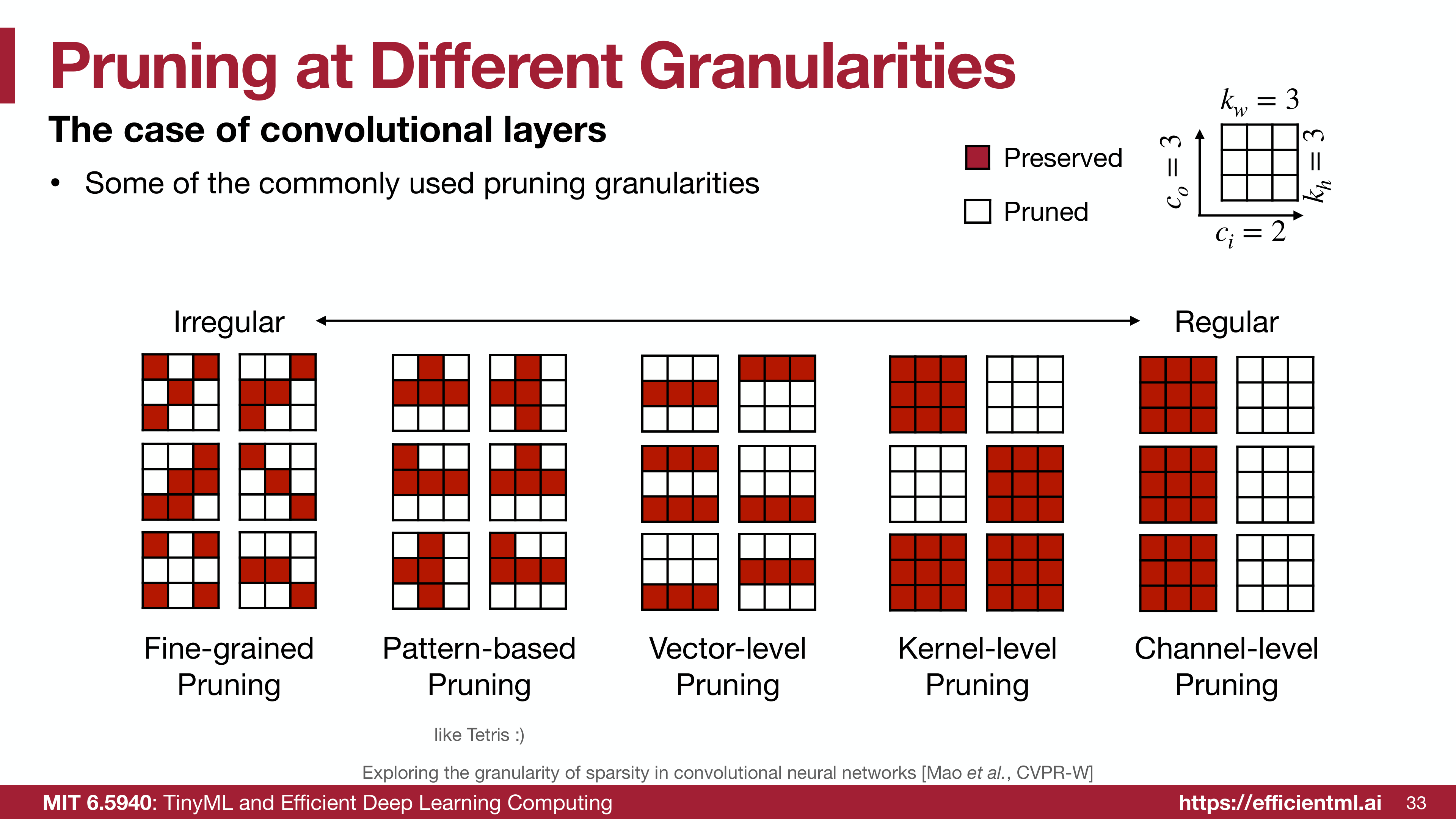
Different pruning granularities from fine to coarse (left to right)

Channel Pruning in Detail

Channel pruning removes entire output channels (filters), which is the most common structured pruning approach.

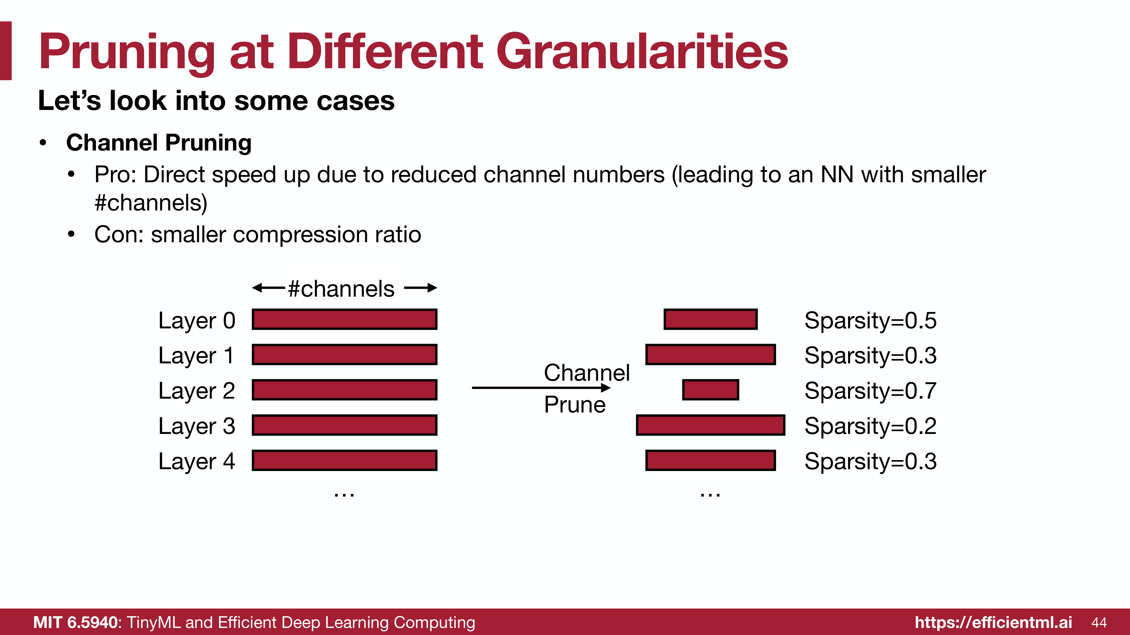
Channel pruning removes entire filters based on their importance

How it works:

1. Before pruning: Network has $N$ channels
2. Evaluate importance of each channel
3. Remove low-importance channels
4. Result: Smaller network with fewer channels

Example:

# Original layer
Conv2d(64 channels -> 128 channels, 3×3 kernel)
Parameters: 64 × 128 × 3 × 3 = 73,728

# After 50% channel pruning
Conv2d(64 channels -> 64 channels, 3×3 kernel)
Parameters: 64 × 64 × 3 × 3 = 36,864

# Reduction: 2× smaller, 2× faster!

Uniform vs. Non-Uniform Pruning

When pruning channels, we have two strategies:

1. Uniform Pruning: Same % pruned from all layers

Layer 0: 50% pruned
Layer 1: 50% pruned
Layer 2: 50% pruned
...

2. Non-Uniform (Adaptive) Pruning: Different % per layer

Layer 0: 30% pruned
Layer 1: 70% pruned
Layer 2: 50% pruned
...

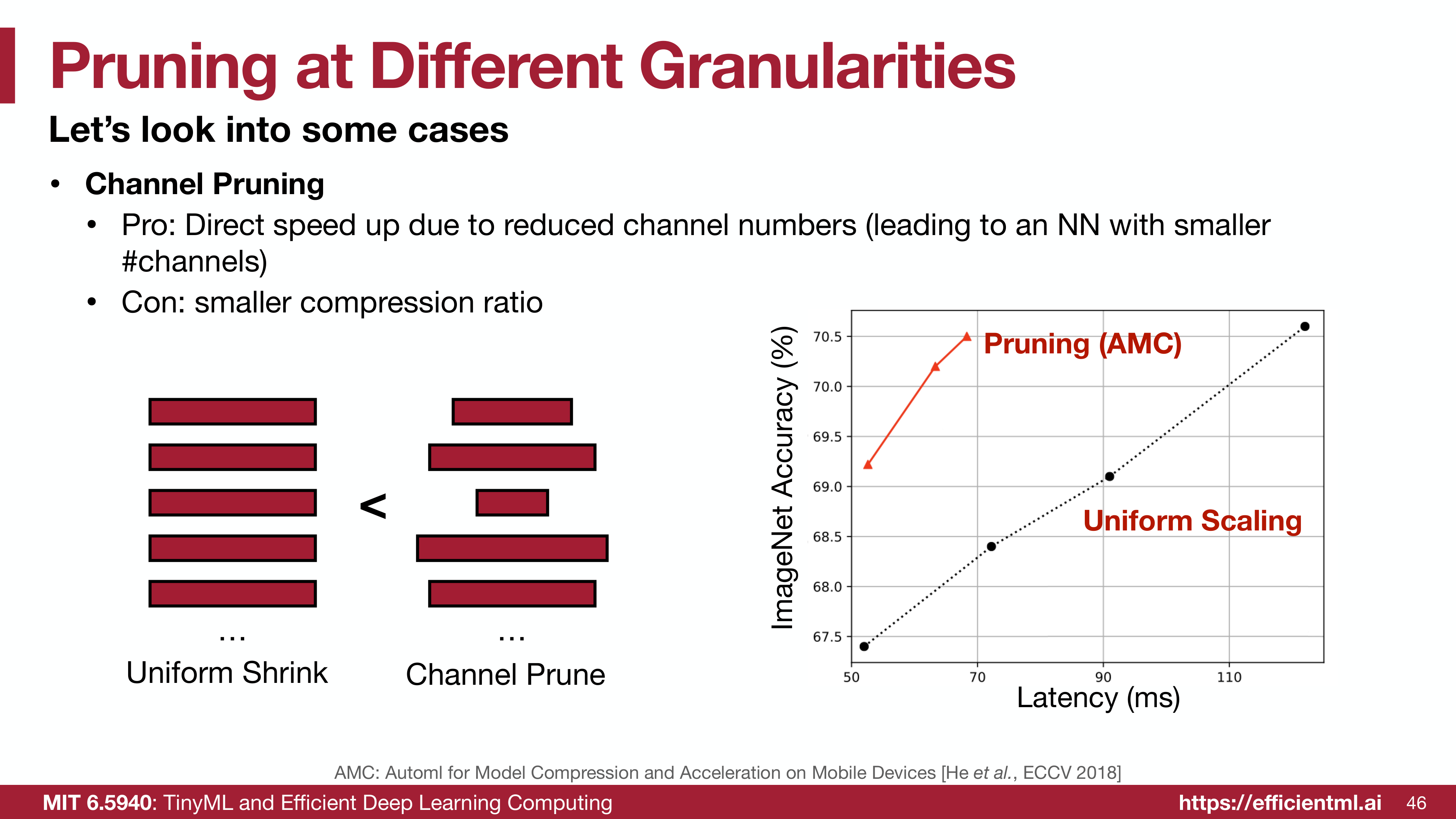
Non-uniform pruning (AMC) outperforms uniform scaling at the same latency

Why non-uniform works better:

• Different layers have different redundancy levels
• Early layers often learn general features (less redundant)
• Later layers learn specific features (more redundant)
• Adaptive methods (like AMC) find optimal per-layer ratios

Pros and Cons of Structured Pruning

Advantages: Direct speedup on any hardware (GPU, CPU, mobile)
No special libraries or hardware needed
Clean, regular structure makes deployment easy
Reduced memory bandwidth requirements
Compatible with quantization and other techniques

Disadvantages: Lower compression ratios (typically 2-5×)
Less flexible in choosing what to prune
May require more careful tuning to maintain accuracy
Coarser granularity means less ability to capture fine-grained redundancy

Comparing All Granularities

Let’s summarize the spectrum:

Granularity	Compression	GPU Speedup	Hardware Requirements	Use Case
Fine-grained	9-12×	None (without custom HW)	Specialized (EIE)	Maximum compression
Pattern (2:4)	2×	~1.5-2×	Modern GPUs (A100+)	Balanced approach
Channel	2-5×	Direct	Any hardware	Production deployment
Layer	2-3×	Direct	Any hardware	Extreme simplification

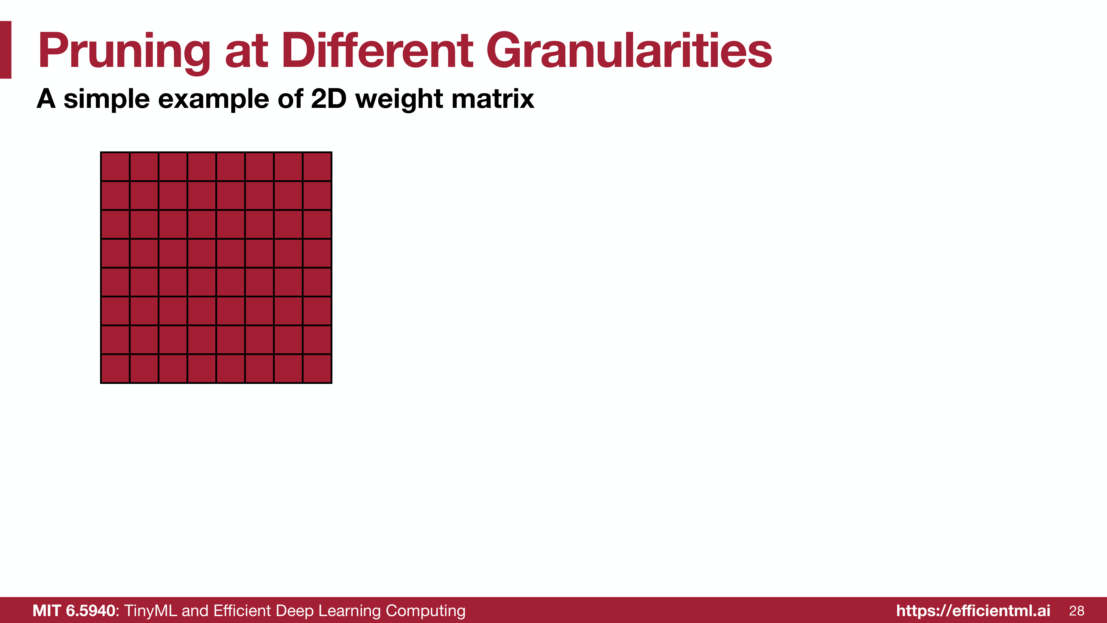
Simple 2D weight matrix showing how different granularities affect the structure

Which Granularity Should You Choose?

Decision Guide

Choose Fine-Grained if:

• You need maximum compression (>10×)
• You have specialized hardware (EIE, sparse tensor cores)
• Model size is your primary constraint
• You can tolerate no speedup on standard GPUs

Choose Pattern-Based (2:4) if:

• You use NVIDIA A100 or newer GPUs
• You want 2× compression with actual speedup
• You need a balance between compression and speed
• You can retrain with sparsity constraints

Choose Channel Pruning if:

• You need to deploy on standard hardware
• Inference speed is critical
• You want simple deployment (no special libraries)
• You’re OK with 2-5× compression

Choose Layer Pruning if:

• You need extreme simplification
• Your model has many similar layers
• You’re working with transformers or ResNets
• You want to combine with other techniques

Real-World Example: Pruning ResNet-50

Let’s see how different granularities affect ResNet-50:

Original:

• Parameters: 25.6M
• FLOPs: 4.1B
• ImageNet Top-1: 76.1%

Fine-grained (90% sparsity):

• Parameters: 2.56M (10×)
• FLOPs: 4.1B (no reduction)
• Top-1: 75.8%
• GPU speedup: None

2:4 Pattern (50% sparsity):

• Parameters: 12.8M (2×)
• FLOPs: 2.05B (2×)
• Top-1: 75.5%
• GPU speedup: 1.5×

Channel Pruning (50% channels):

• Parameters: 6.4M (4×)
• FLOPs: 1.03B (4×)
• Top-1: 73.2%
• GPU speedup: 3.8×

Key Takeaways

1. Pruning granularity creates a trade-off between compression ratio and hardware efficiency
2. Fine-grained pruning achieves highest compression but requires special hardware
3. Pattern-based (2:4) pruning is hardware-accelerated on modern GPUs
4. Channel pruning works on any hardware and provides direct speedup
5. Non-uniform pruning (different ratios per layer) outperforms uniform pruning
6. The right choice depends on your deployment target and constraints

What’s Next?

We’ve learned what patterns to prune in, but we haven’t answered a crucial question: Which specific weights or channels should we remove?

In Part 3, we’ll explore pruning criteria—the methods that determine which parameters are important and which can be safely removed.

---

Series Navigation:

• Part 1: Why Pruning Matters
• Part 2: Pruning Granularities (Current)
• Part 3: Pruning Criteria
• Part 4: Advanced Techniques

References:

• MIT 6.5940: TinyML and Efficient Deep Learning (Fall 2024)
• Learning Both Weights and Connections for Efficient Neural Network (Han et al., NeurIPS 2015)
• Exploring the Granularity of Sparsity in CNNs (Mao et al., CVPR 2017)
• Accelerating Inference with Sparsity Using NVIDIA Ampere
• AMC: AutoML for Model Compression (He et al., ECCV 2018)