Neural Network Pruning Part 4: Advanced Techniques and Practical Applications

The Journey So Far

Throughout this series, we’ve built a comprehensive understanding of neural network pruning:

• Part 1: Why pruning matters (model size explosion, energy costs)
• Part 2: What patterns to prune (fine-grained, pattern-based, structured)
• Part 3: Which parameters to remove (magnitude, scaling, second-order)

Now we tackle the final pieces: How much to prune, how to train pruned networks, and how to automate the entire process.

The Pruning Ratio Challenge

The Core Question

Once we know what granularity and which criterion to use, we face a critical decision:

How much should we prune from each layer?

This isn’t just one number—different layers have different redundancy levels.

The Naive Approach: Uniform Pruning

Uniform pruning applies the same pruning ratio to all layers:

# Uniform 50% pruning
for layer in network:
    prune_layer(layer, ratio=0.5)

Example:

Layer 0 (conv1): 50% pruned
Layer 1 (conv2): 50% pruned
Layer 2 (conv3): 50% pruned
...
Layer N (fc):    50% pruned

Why Uniform Pruning Falls Short

Different layers play different roles:

Early layers (close to input):

• Learn general features (edges, textures)
• Less redundant
• More sensitive to pruning

Middle layers:

• Learn intermediate features
• Moderate redundancy

Late layers (close to output):

• Learn task-specific features
• Often highly redundant
• More tolerant to aggressive pruning

Analogy: It’s like cutting the same percentage of budget from every department—it ignores that some departments have more waste than others.

The Better Approach: Layer-wise Pruning Ratios

Layer-wise pruning assigns different ratios per layer:

pruning_ratios = {
    'layer0': 0.30,  # Early layer: prune less
    'layer1': 0.45,
    'layer2': 0.60,
    'layer3': 0.70,  # Late layer: prune more
    'fc':     0.85   # Fully connected: very redundant
}

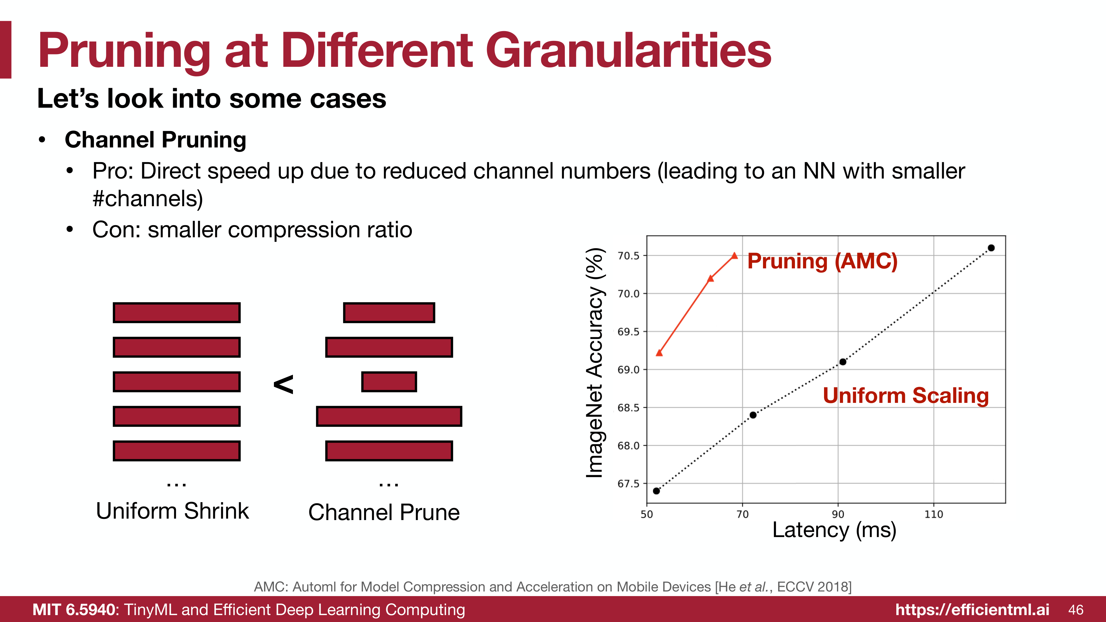
Layer-wise adaptive pruning (AMC) significantly outperforms uniform scaling

Sensitivity Analysis

To find good layer-wise ratios, perform sensitivity analysis:

1. For each layer independently:
   • Prune at different ratios (10%, 20%, …, 90%)
   • Measure accuracy drop
2. Plot sensitivity curves:
   • X-axis: Pruning ratio
   • Y-axis: Accuracy drop
3. Identify tolerance:
   • Flat curves = tolerant to pruning
   • Steep curves = sensitive to pruning

Example results:

Layer 1: Accuracy drops 5% at 80% pruning   → Tolerant
Layer 5: Accuracy drops 20% at 50% pruning  → Sensitive
Layer 10: Accuracy drops 2% at 90% pruning  → Very tolerant

Strategy: Prune more from tolerant layers, less from sensitive ones.

Iterative Pruning: The Secret Sauce

One-Shot vs. Iterative Pruning

One-shot pruning:

1. Train network
2. Prune to target sparsity (e.g., 90%)
3. Fine-tune
4. Done

Problem: Large pruning in one step causes significant accuracy drop.

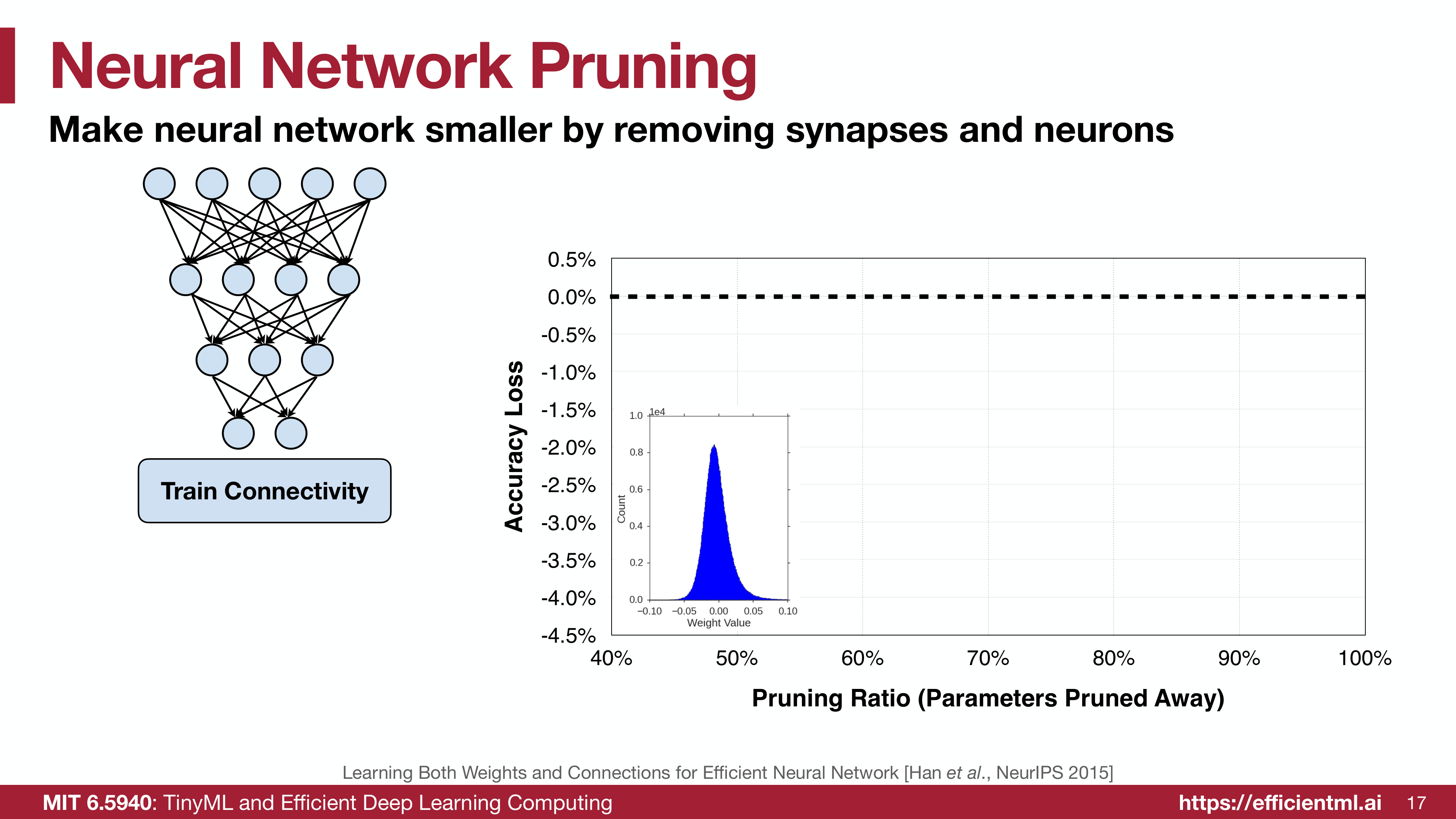
Iterative pruning with fine-tuning dramatically outperforms one-shot pruning

The Iterative Pruning Algorithm

Iterative pruning prunes gradually:

# Iterative pruning (pseudo-code)
model = train_model()
target_sparsity = 0.90
current_sparsity = 0.0
step_size = 0.10  # Prune 10% at a time

while current_sparsity < target_sparsity:
    # Prune a small amount
    prune_weights(model, sparsity=current_sparsity + step_size)
    current_sparsity += step_size
    
    # Fine-tune to recover accuracy
    fine_tune(model, epochs=5)
    
    # Evaluate
    accuracy = evaluate(model)
    print(f"Sparsity: {current_sparsity:.0%}, Accuracy: {accuracy:.2%}")

Why Iterative Works Better

Intuition: It’s like gradually reducing food intake to lose weight vs. suddenly starving yourself.

Technical reasons:

1. Smaller disturbance per step: Network stays close to good optimum
2. Fine-tuning recovers accuracy: Remaining weights compensate
3. Network adapts gradually: Learns to work with fewer parameters
4. Exploration of loss landscape: Finds better sparse solutions

Practical Example: ResNet-50

One-shot 90% pruning:

• Accuracy drop: 15%
• Fine-tuning recovers: 8%
• Final accuracy loss: 7%

Iterative 90% pruning (9 iterations of 10%):

• Accuracy drop per iteration: ~2%
• Fine-tuning recovers: 1.5%
• Cumulative effect: <1% final loss

Looking ahead: Iterative pruning works remarkably well, but it still assumes we need to train dense first. What if sparse networks could train from scratch? We’ll explore this radical idea in Part 5 with the Lottery Ticket Hypothesis.

Automated Pruning: AutoML for Compression

The Manual Problem

Finding optimal pruning ratios manually is:

• Time-consuming (try many combinations)
• Requires expertise (know which layers are important)
• Suboptimal (hard to find global optimum)
• Tedious (repeat for every architecture)

Solution: Automate the search with AutoML for Model Compression (AMC).

AMC: Reinforcement Learning for Pruning

The Idea: Use an RL agent to learn optimal pruning ratios for each layer.

Components:

1. Agent (Policy Network):

• Takes layer features as input (# channels, position, etc.)
• Outputs pruning ratio for that layer

2. Environment (Network + Dataset):

• Agent prunes network according to its policy
• Measures accuracy and model size

3. Reward Function:

reward = accuracy - λ * (model_size / target_size)

Where:

• High accuracy → positive reward
• Smaller size → bonus reward
• Missing target → penalty

4. Training Process:

1. Agent proposes pruning ratios
2. Prune network according to ratios
3. Fine-tune and measure performance
4. Calculate reward
5. Update agent to maximize future reward
6. Repeat

AMC Results

AMC finds pruning ratios that dominate uniform scaling on the accuracy-latency curve

MobileNet-V1 on ImageNet:

Method	Top-1 Accuracy	Latency (ms)	Speedup
Baseline	70.6%	113	1.0×
Uniform 50%	68.2%	75	1.5×
AMC 50%	70.5%	60	1.9×

AMC achieves:

• Same accuracy as baseline
• 1.9× faster inference
• Better than naive uniform pruning

Beyond AMC: Other Automated Approaches

1. Neural Architecture Search (NAS):

• Search over channel numbers directly
• More general than pruning
• Higher computational cost

2. Differentiable Pruning:

• Make pruning ratios continuous and differentiable
• Use gradient descent to optimize
• Faster than RL-based methods

3. Lottery Ticket Hypothesis:

• Find “winning lottery tickets” (sparse subnetworks)
• Train from scratch with found mask
• Can match dense performance

Training Pruned Networks: Best Practices

Fine-tuning Strategies

Strategy 1: Standard Fine-tuning

# After pruning
optimizer = SGD(model.parameters(), lr=0.001)
train(model, epochs=10)

Strategy 2: Gradual Unfreezing

# Unfreeze layers gradually
for layer_group in reversed(model.layers):
    unfreeze(layer_group)
    train(model, epochs=2)

Strategy 3: Learning Rate Warmup

# Start with small LR, gradually increase
scheduler = WarmupScheduler(initial_lr=1e-5, target_lr=1e-2, warmup_epochs=5)
train(model, epochs=20, scheduler=scheduler)

Advanced training techniques like learning rate rewinding and sparse training from scratch are covered in depth in Part 5.

Combining Pruning with Other Techniques

Pruning + Quantization:

Original: 100M params × 32 bits = 3.2 GB
After pruning (10×): 10M params × 32 bits = 320 MB
After quantization (INT8): 10M params × 8 bits = 80 MB

Total compression: 40×

Pruning + Knowledge Distillation:

1. Train large teacher network
2. Prune to create student
3. Distill knowledge from teacher to student
4. Student learns from both data and teacher

Pruning + Low-Rank Factorization:

# Original layer
W ∈ R^(1000×1000)  →  1M parameters

# Prune to 50%
W_sparse  →  500K parameters

# Further compress with low-rank
W ≈ U × V, where U ∈ R^(1000×100), V ∈ R^(100×1000)
→  200K parameters

Total: 5× compression

Real-World Applications and Case Studies

Case Study 1: MLPerf Inference (2024)

Task: Optimize Llama 2 70B for inference

Approach:

• Depth pruning: 80 layers → 32 layers (60% reduction)
• Width pruning: 28,762 → 14,336 intermediate dims (50% reduction)
• Fine-tuning on large-scale dataset

Results:

• 2.5× speedup in inference
• 99% accuracy retention
• Deployed on NVIDIA H200 GPU

Case Study 2: Mobile Deployment

Task: Deploy ResNet-50 on smartphone

Challenges:

• Limited memory (< 100 MB for model)
• Low power budget
• Real-time inference (< 50 ms)

Solution:

• Channel pruning (60% of channels)
• Iterative pruning with 10 rounds
• INT8 quantization
• Result: 25 MB model, 30 ms latency

Case Study 3: Image Captioning with LSTM

Baseline NeuralTalk LSTM:

• Parameters: 100M
• Inference: 200 ms/image

After 90% pruning:

• Parameters: 10M (10× smaller)
• Inference: 120 ms/image (1.7× faster)
• Caption quality: Maintained!

Example captions:

Image: Basketball player
Baseline: "a basketball player in a white uniform is playing with a ball"
Pruned:   "a basketball player in a white uniform is playing with a basketball"

Image: Dog in field
Baseline: "a brown dog is running through a grassy field"
Pruned:   "a brown dog is running through a grassy area"

Both capture the essential content!

Practical Implementation Guide

Step-by-Step Pruning Pipeline

1. Baseline Training

# Train your model normally first
model = ResNet50()
train(model, epochs=90)
baseline_accuracy = evaluate(model)
print(f"Baseline: {baseline_accuracy:.2%}")

2. Sensitivity Analysis

# Test each layer's sensitivity
for layer_name, layer in model.named_modules():
    sensitivities[layer_name] = []
    for ratio in [0.1, 0.3, 0.5, 0.7, 0.9]:
        pruned = prune_layer(layer, ratio)
        acc = evaluate(model)
        sensitivities[layer_name].append((ratio, acc))

3. Determine Layer-wise Ratios

# Allocate pruning ratios based on sensitivity
target_sparsity = 0.7
ratios = {}
for layer_name in model.layers:
    if sensitivities[layer_name] < threshold:
        ratios[layer_name] = 0.8  # Tolerant → prune more
    else:
        ratios[layer_name] = 0.5  # Sensitive → prune less

4. Iterative Pruning

# Gradual pruning with fine-tuning
for iteration in range(10):
    # Prune 10% more
    current_target = 0.1 * (iteration + 1) * target_sparsity
    prune_network(model, ratios, target=current_target)
    
    # Fine-tune
    fine_tune(model, epochs=5, lr=1e-3)
    
    # Evaluate
    acc = evaluate(model)
    print(f"Iteration {iteration}, Sparsity: {current_target:.1%}, "
          f"Accuracy: {acc:.2%}")

5. Final Fine-tuning

# Longer fine-tuning at the end
fine_tune(model, epochs=20, lr_schedule=cosine_schedule)
final_accuracy = evaluate(model)
print(f"Final: {final_accuracy:.2%} (drop: {baseline_accuracy - final_accuracy:.2%})")

Tools and Libraries

PyTorch:

import torch.nn.utils.prune as prune

# Magnitude pruning
prune.l1_unstructured(module, name='weight', amount=0.5)

# Structured pruning
prune.ln_structured(module, name='weight', amount=0.3, n=2, dim=0)

TensorFlow:

import tensorflow_model_optimization as tfmot

# Pruning schedule
pruning_schedule = tfmot.sparsity.keras.PolynomialDecay(
    initial_sparsity=0.0,
    final_sparsity=0.8,
    begin_step=0,
    end_step=1000
)

# Apply pruning
model = tfmot.sparsity.keras.prune_low_magnitude(model, pruning_schedule)

Specialized Libraries:

• Neural Network Intelligence (NNI): Microsoft’s AutoML toolkit
• Distiller: Intel’s pruning library
• PocketFlow: Tencent’s model compression framework

Common Pitfalls and How to Avoid Them

Pitfall 1: Pruning Too Aggressively

Problem: Removing 90% of parameters in one shot

Solution: Use iterative pruning (5-10 iterations)

Pitfall 2: Ignoring Layer Sensitivity

Problem: Uniform pruning hurts critical layers

Solution: Perform sensitivity analysis, use layer-wise ratios

Pitfall 3: Insufficient Fine-tuning

Problem: Fine-tuning for only 1-2 epochs

Solution: Fine-tune for 10-20% of original training time

Pitfall 4: Wrong Learning Rate

Problem: Using very small LR for fine-tuning

Solution: Use learning rate rewinding or moderate LR (1e-3 to 1e-2)

Pitfall 5: Not Measuring Real Speedup

Problem: Assuming 10× parameter reduction = 10× speedup

Reality: Fine-grained pruning may have no speedup on GPUs

Solution: Measure actual inference time on target hardware

Key Takeaways

1. Layer-wise pruning ratios outperform uniform pruning
2. Iterative pruning with fine-tuning is essential for high sparsity
3. AutoML methods (AMC) can find better ratios than manual search
4. Combining pruning with quantization achieves extreme compression (40-50×)
5. Real-world deployment requires measuring actual speedup on target hardware
6. Different applications need different strategies (mobile vs. cloud vs. edge)
7. Pruning is production-ready with hardware support and proven results

Conclusion: The Path Forward

We’ve covered the practical foundations of neural network pruning:

What We Know:

1. Layer-wise pruning beats uniform pruning
2. Iterative approach with fine-tuning is essential
3. AutoML (AMC) can automate ratio selection
4. Combining techniques (pruning + quantization) maximizes compression
5. Real hardware validation is critical for deployment

What This Achieves:

• 3-12× model compression
• 2-5× inference speedup (with structured pruning)
• 50-100× memory reduction (with pruning + quantization)

But this raises deeper questions:

• Why does pruning work so well?
• Do we actually need dense networks for training?
• Can we train sparse networks from scratch?

In Part 5, we’ll explore the Lottery Ticket Hypothesis and modern sparse training methods that challenge everything we thought we knew about pruning.

---

Series Navigation:

• Part 1: Why Pruning Matters
• Part 2: Pruning Granularities
• Part 3: Pruning Criteria
• Part 4: Advanced Techniques (Current)
• Part 5: Lottery Tickets and Beyond

References:

• MIT 6.5940: TinyML and Efficient Deep Learning (Fall 2024)
• Original Pruning Paper (Han et al., NeurIPS 2015)
• AMC: AutoML for Model Compression
• Deep Compression (Han et al., ICLR 2016)
• To Prune, or Not to Prune: Exploring the Efficacy of Pruning