Neural Network Pruning Part 3: Pruning Criteria

Recap: The Pattern is Set, But Which Weights?

In Part 2, we learned about different pruning granularities—from fine-grained to structured. Now we face the critical question:

Which specific weights, channels, or neurons should we remove?

Imagine you’re a gardener pruning a rose bush. You know you want to cut branches (granularity), but which ones? The dead branches? The small ones? The ones pointing inward? The criterion you use determines whether your roses thrive or die.

Similarly, in neural networks, using the right pruning criterion means the difference between maintaining accuracy and destroying your model’s performance.

The Core Challenge

When removing parameters from a neural network, our goal is:

Remove the least important parameters while preserving the most important information.

But what makes a parameter “important”?

Simple Example

Consider a simple neuron:

\[y = f(w_0 x_0 + w_1 x_1 + w_2 x_2 + b)\]

With weights: $W = [10, -8, 0.1]$ and activation $f = \text{ReLU}$

\[y = \text{ReLU}(10x_0 - 8x_1 + 0.1x_2 + b)\]

Question: If you must remove one weight, which one?

Intuitively, $w_2 = 0.1$ seems least important—it has minimal impact on the output. But is magnitude always the best criterion? Let’s explore.

Pruning Criterion #1: Magnitude-Based Pruning

The Core Idea

Magnitude-based pruning assumes that weights with larger absolute values are more important than those with smaller absolute values.

Intuition: A weight of 10 has much more impact on the output than a weight of 0.01, so we keep the large one.

Element-wise Magnitude Pruning

For removing individual weights:

\[\text{Importance}(w_i) = |w_i|\]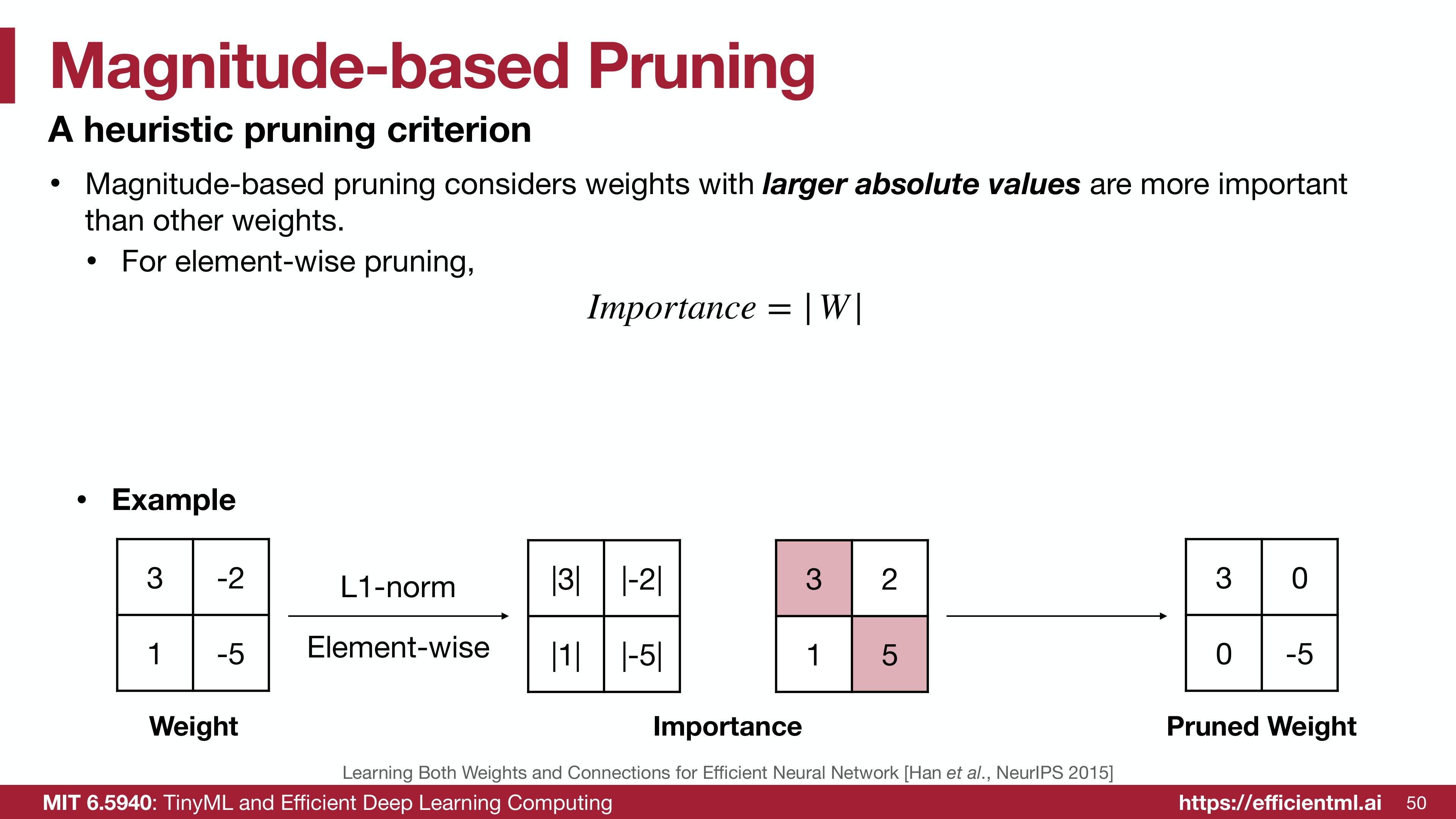

Example: Element-wise magnitude pruning removes weights with smallest absolute values

Example:

Original weights: [3, -2, 1, -5]
Magnitudes:       [3,  2, 1,  5]

# Keep top 50% by magnitude
Pruned weights:   [3,  0, 0, -5]

Notice that both positive and negative values are preserved if their magnitude is large.

L1-Norm for Structured Pruning

When pruning groups (like rows, channels), we need a criterion for the entire group:

\[\text{Importance}(W_S) = \sum_{i \in S} |w_i|\]

Where $S$ is the set of weights in the structure (e.g., a channel).

Example: Row-wise pruning

Weight matrix:
Row 0: [3, -2]  →  L1-norm = |3| + |-2| = 5
Row 1: [1, -5]  →  L1-norm = |1| + |-5| = 6

# Row 0 has smaller L1-norm, so it's pruned
Pruned matrix:
Row 0: [0,  0]
Row 1: [1, -5]

L2-Norm Alternative

We can also use L2-norm (Euclidean distance):

\[\text{Importance}(W_S) = \sqrt{\sum_{i \in S} w_i^2}\]

Example: Same matrix with L2-norm

Row 0: [3, -2]  →  L2-norm = √(9 + 4) = √13 ≈ 3.61
Row 1: [1, -5]  →  L2-norm = √(1 + 25) = √26 ≈ 5.10

# Row 0 still has smaller norm, so it's pruned

L1 vs L2:

• L1: More robust to outliers, sparse-promoting
• L2: Standard in most frameworks, smoother

Pros and Cons

Advantages: Extremely simple to implement (one line of code)
No additional training or data required
Fast computation (just sort weights)
Works surprisingly well in practice
Hardware-agnostic

Disadvantages: Ignores activation values (what if $x_0$ is always near zero?)
Doesn’t consider second-order effects
Assumes magnitude = importance (not always true)
Sensitive to weight initialization scale

When to Use It

Magnitude-based pruning is your go-to baseline:

• Quick experiments and prototyping
• Post-training pruning (no retraining budget)
• When you need a simple, reliable method
• Initial pruning before fine-tuning

Pruning Criterion #2: Scaling-Based Pruning

The Core Idea

Instead of looking at raw weight magnitudes, train a scaling factor for each channel/filter that indicates its importance.

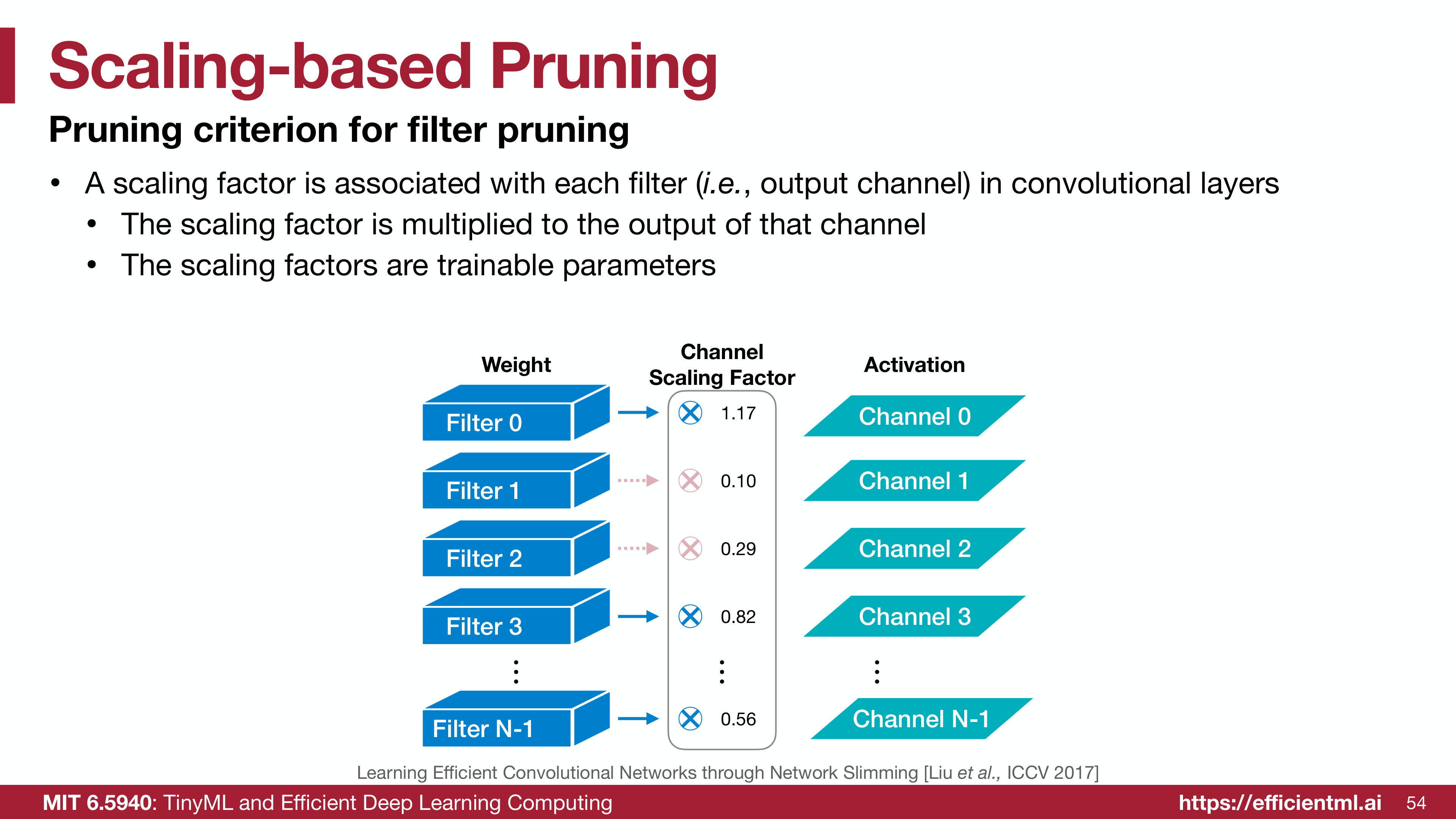
Each channel has a learnable scaling factor that modulates its output

How It Works

1. Add a scaling factor $\gamma$ to each channel:

\[z_{\text{out}} = \gamma \cdot f(W \cdot x)\]

1. Train the network with these scaling factors
2. Apply L1 regularization on $\gamma$ to encourage sparsity:

\[\mathcal{L}_{\text{total}} = \mathcal{L}_{\text{task}} + \lambda \sum_{c} |\gamma_c|\]

1. Prune channels with small $

   \gamma

   $ values

Connection to Batch Normalization

If your network uses Batch Normalization (BN), you already have scaling factors!

\[\text{BN output: } z_{\text{out}} = \gamma \frac{z_{\text{in}} - \mu}{\sqrt{\sigma^2 + \epsilon}} + \beta\]

The $\gamma$ parameters in BN can directly serve as importance indicators.

Practical approach:

1. Fine-tune network with L1 regularization on BN’s $\gamma$

2. Prune channels where $

   \gamma

   $ < threshold

3. Fine-tune pruned network

Example

# Before pruning
Channel 0: γ = 1.17  Keep
Channel 1: γ = 0.10  Prune
Channel 2: γ = 0.29  Prune
Channel 3: γ = 0.82  Keep

# After pruning (50% target)
Network now has 2 channels instead of 4

Pros and Cons

Advantages: End-to-end learnable importance scores
Leverages existing BN parameters (no extra overhead)
Considers full training dynamics
Better than magnitude for structured pruning
Regularization encourages sparsity during training

Disadvantages: Requires retraining with regularization
Only works for structured pruning (channels/filters)
Hyperparameter tuning needed (λ for regularization)
Assumes BN is present (doesn’t work for all architectures)

When to Use It

Scaling-based pruning is ideal for:

• Channel/filter pruning in CNNs
• When you have batch normalization
• When you can afford retraining
• For achieving structured sparsity

Pruning Criterion #3: Second-Order Methods

The Core Idea

Instead of heuristics (magnitude), let’s answer: What is the actual impact on the loss function when we remove a parameter?

This leads to Optimal Brain Damage (OBD), a classic method from 1989 that’s still influential today.

The Math Behind It

When we remove weight $w_i$ (set it to 0), the change in loss is:

\[\delta L = L(W) - L(W_{\text{pruned}}) = L(W) - L(W - \delta W)\]

Using a Taylor series expansion around the current weights:

\[\delta L = \sum_i g_i \delta w_i + \frac{1}{2} \sum_i h_{ii} \delta w_i^2 + \frac{1}{2} \sum_{i \neq j} h_{ij} \delta w_i \delta w_j + O(||\delta W||^3)\]

Where:

• $g_i = \frac{\partial L}{\partial w_i}$ (first-order gradient)
• $h_{ij} = \frac{\partial^2 L}{\partial w_i \partial w_j}$ (second-order Hessian)

Optimal Brain Damage Assumptions

To make this computationally tractable, OBD makes three assumptions:

Assumption 1: Network has converged

• Gradients $g_i \approx 0$
• Eliminates first-order terms

Assumption 2: Loss is quadratic

• Higher-order terms $O(

  \delta W

  ^3)$ negligible

Assumption 3: Parameters are independent

• Off-diagonal Hessian terms $h_{ij} = 0$ for $i \neq j$

With these assumptions:

\[\delta L_i \approx \frac{1}{2} h_{ii} w_i^2\]

The Importance Criterion

\[\text{Importance}(w_i) = \frac{1}{2} h_{ii} w_i^2\]

Where $h_{ii}$ is the diagonal element of the Hessian matrix.

Interpretation:

• **Large $

  w_i

  $**: Weight has large magnitude (like magnitude pruning)

• Large $h_{ii}$: Weight is in a “sensitive” region of loss landscape
• Combined: Captures both magnitude AND curvature information

Why It’s Better Than Magnitude

Consider two weights:

• $w_1 = 0.5$ in a flat region ($h_{11} = 0.1$): Importance = $0.5 \times 0.1 \times 0.25 = 0.0125$
• $w_2 = 0.3$ in a steep region ($h_{22} = 2.0$): Importance = $0.5 \times 2.0 \times 0.09 = 0.09$

Pure magnitude would prune $w_2$, but OBD correctly identifies that $w_1$ is less important despite being larger!

Practical Challenges

The Hessian Problem:

• For a network with $N$ parameters, Hessian is $N \times N$ matrix
• ResNet-50 has 25M parameters → Hessian would be 625 trillion entries!
• Computing and storing the full Hessian is infeasible

Approximations:

• Compute only diagonal elements $h_{ii}$
• Use Fisher Information Matrix as approximation
• Employ low-rank approximations

Pros and Cons

Advantages: Theoretically principled (minimizes loss increase)
Captures curvature information (not just magnitude)
Better accuracy than magnitude-based methods
Considers loss landscape geometry

Disadvantages: Computationally expensive (Hessian calculation)
Memory intensive for large networks
Requires assumptions that may not hold
Complex implementation

When to Use It

Second-order methods are worth it when:

• You need the best possible accuracy retention
• You can afford the computational cost
• You’re pruning critical models (medical, safety-critical)
• You’re doing research and need optimal results

Pruning Criterion #4: Gradient-Based Methods

The Core Idea

Similar to second-order methods, but uses gradients of the loss with respect to removing parameters.

For a parameter $w_i$, compute:

\[\text{Importance}(w_i) = \left| \frac{\partial L}{\partial w_i} \right| \cdot |w_i|\]

Interpretation:

• Large gradient: Loss is sensitive to changes in this weight
• Large weight: Weight has significant magnitude
• Product captures both aspects

Taylor Series Pruning

A recent variant uses first-order Taylor expansion:

\[\delta L \approx \sum_i \frac{\partial L}{\partial w_i} \cdot \delta w_i\]

For pruning (setting $w_i = 0$, so $\delta w_i = -w_i$):

\[\text{Importance}(w_i) = \left| \frac{\partial L}{\partial w_i} \cdot w_i \right|\]

Pros and Cons

Advantages: Cheaper than second-order methods
More accurate than pure magnitude
Considers loss sensitivity
Easy to implement with auto-diff

Disadvantages: Requires forward/backward pass on data
Can be noisy (depends on batch)
Not as accurate as second-order

Pruning Criterion #5: Activation-Based Methods

The Core Idea

Instead of looking at weights, look at the activations they produce.

Key Insight: If a neuron’s output is frequently zero (after ReLU), it’s not contributing much to the network.

Average Percentage of Zeros (APoZ)

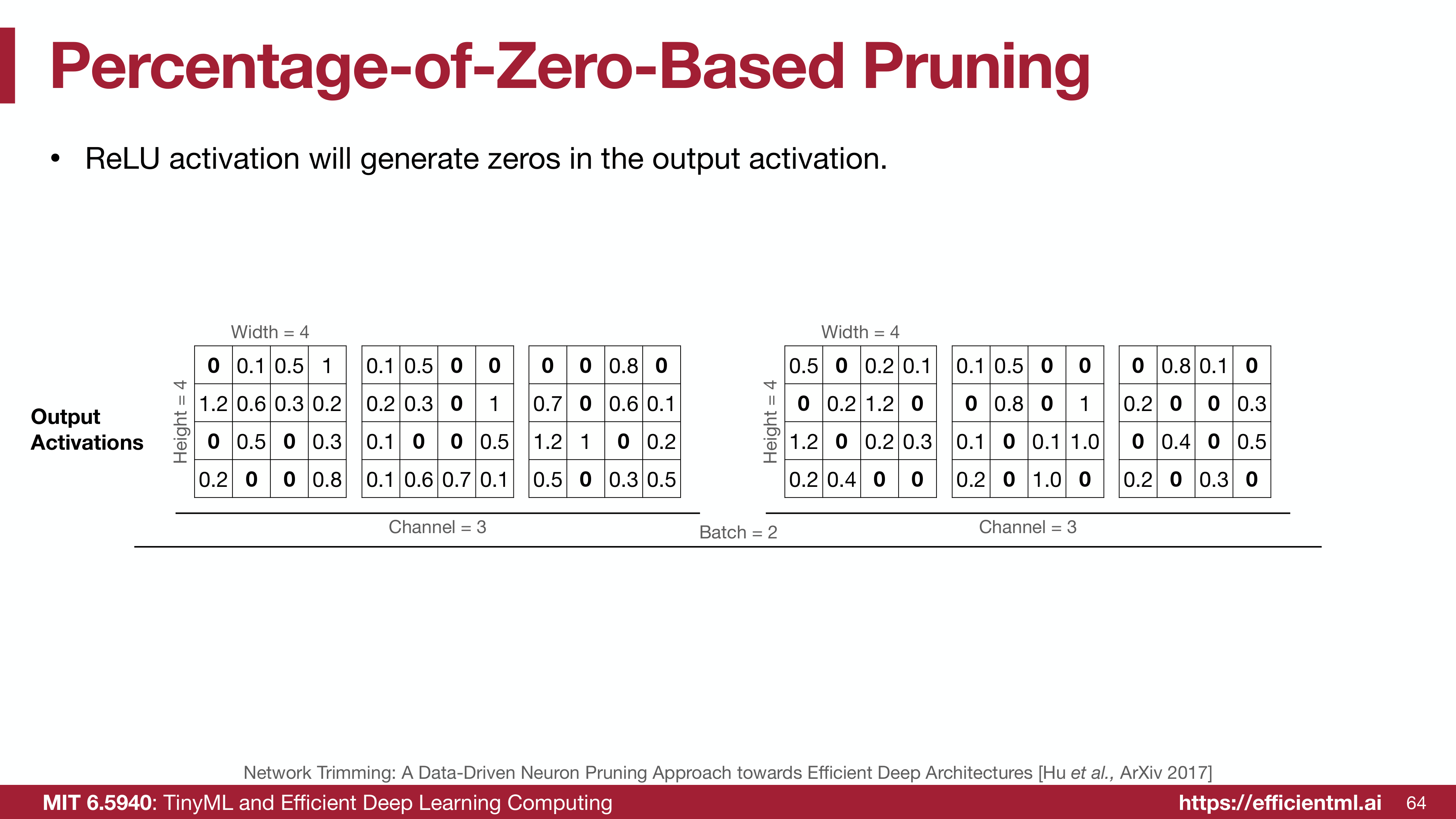
Computing Average Percentage of Zeros across multiple samples and spatial locations

For a channel $c$, across $B$ samples and $H \times W$ spatial locations:

\[\text{APoZ}_c = \frac{1}{B \times H \times W} \sum_{b=1}^{B} \sum_{h=1}^{H} \sum_{w=1}^{W} \mathbb{1}[a_{c,h,w}^{(b)} = 0]\]

Where $\mathbb{1}[\cdot]$ is the indicator function (1 if true, 0 otherwise).

Example:

Channel 0: 11/32 zeros → APoZ = 34%  ✓ Keep
Channel 1: 12/32 zeros → APoZ = 38%  ✓ Keep
Channel 2: 14/32 zeros → APoZ = 44%  ✗ Prune

Why It Works

High APoZ means:

• Neuron is frequently inactive
• Not contributing to many predictions
• Likely redundant

Low APoZ means:

• Neuron is frequently active
• Contributing to many predictions
• Likely important

Pros and Cons

Advantages: Data-driven (uses actual activations)
No gradient computation required
Works well for ReLU networks
Captures runtime behavior
Simple to implement

Disadvantages: Requires forward passes on calibration data
Specific to ReLU and similar activations
Can be biased by calibration data selection
Doesn’t work for all activation functions

When to Use It

Activation-based methods are great for:

• Post-training pruning (no gradients needed)
• When you have representative calibration data
• ReLU-based networks (CNNs)
• Structured pruning (neurons/channels)

Pruning Criterion #6: Regression-Based Methods

The Core Idea

Instead of minimizing the change in final loss, minimize the reconstruction error at each layer.

Analogy: Rather than worrying about the final exam score, make sure each chapter’s summary is accurate.

The Formulation

For layer $l$ with output $Z$:

\[Z = X W^T\]

After pruning, we want pruned output $\hat{Z}$ to be close to original:

\[\min_{W_P} \|Z - \hat{Z}\|_F^2 = \min_{W_P} \|Z - X W_P^T\|_F^2\]

Channel Selection Problem

For channel pruning, we introduce binary indicators $\beta_c$:

\[\min_{W, \beta} \left\| Z - \sum_{c=1}^{C} \beta_c X_c W_c^T \right\|_F^2\]

Subject to: $|\beta|_0 \leq N$ (at most $N$ channels kept)

Where:

• $\beta_c = 1$: Keep channel $c$
• $\beta_c = 0$: Prune channel $c$

Alternating Optimization

Since the problem is hard to solve directly, use alternating optimization:

Step 1: Fix $W$, solve for $\beta$ (channel selection) Step 2: Fix $\beta$, solve for $W$ (weight optimization)

Repeat until convergence.

Pros and Cons

Advantages: Layer-wise optimization (computationally efficient)
Principled reconstruction objective
Works well for structured pruning
Can combine with other criteria

Disadvantages: Doesn’t consider end-to-end loss
Requires solving optimization problem
May not preserve final task performance
More complex implementation

Comparing All Criteria

Criterion	Complexity	Accuracy	Speed	Best For
Magnitude	Low	Good	Fast	Baseline, fine-grained
Scaling (BN γ)	Medium	Very Good	Medium	Channel pruning
Second-Order	Very High	Excellent	Slow	Research, critical apps
Gradient	Medium	Good	Medium	Balanced approach
Activation (APoZ)	Low	Good	Fast	Post-training, ReLU nets
Regression	High	Very Good	Medium	Structured pruning

Practical Recommendations

For Quick Experiments

Use magnitude-based pruning
Works 80% of the time
Fast to implement and run

For Production Deployment

Use scaling-based (BN γ) for channel pruning
Fine-tune with L1 regularization
Balance accuracy and speed

For Research / Maximum Accuracy

Use second-order methods or gradient-based
Worth the computational cost
Combine with iterative pruning

For Post-Training Compression

Use magnitude or activation-based (APoZ)
No need for gradients
Works with frozen models

Key Takeaways

1. Different criteria measure “importance” differently: magnitude, gradients, activations, reconstruction error
2. Magnitude-based pruning is surprisingly effective and should be your baseline
3. Scaling-based methods (BN γ) work best for structured channel pruning
4. Second-order methods are most accurate but computationally expensive
5. Activation-based methods are data-driven and work well post-training
6. The best criterion depends on your constraints (time, accuracy, hardware)

What’s Next?

We now know what pattern to prune (granularity) and which parameters to remove (criterion). But there are still critical questions:

• How much should we prune from each layer?
• Should we prune all at once or iteratively?
• How do we fine-tune the pruned network?
• Can we automate the entire process?

In Part 4, we’ll explore advanced pruning techniques including iterative pruning, automated pruning ratio search, and combining pruning with other compression methods.

---

Series Navigation:

• Part 1: Why Pruning Matters
• Part 2: Pruning Granularities
• Part 3: Pruning Criteria (Current)
• Part 4: Advanced Techniques

References:

• MIT 6.5940: TinyML and Efficient Deep Learning (Fall 2024)
• Optimal Brain Damage (LeCun et al., NeurIPS 1989)
• Learning Both Weights and Connections (Han et al., NeurIPS 2015)
• Learning Efficient CNNs through Network Slimming (Liu et al., ICCV 2017)
• Network Trimming: Data-Driven Neuron Pruning (Hu et al., 2016)
• Channel Pruning for Accelerating Deep CNNs (He et al., ICCV 2017)