Efficiency Metrics Part 1: Performance Metrics for Deep Learning
Understanding latency and throughput - the key performance metrics for evaluating neural network efficiency
Deep learning models are becoming increasingly powerful, but with great power comes great resource consumption. Understanding how to measure efficiency is crucial for practical deployment. This three-part series explains essential metrics for evaluating neural network efficiency.
What Are Efficiency Metrics?
Efficiency metrics are quantitative measures that help us understand how well a neural network utilizes computational resources. Think of them as the “fuel economy ratings” for deep learning models:
Three Main Categories:
- Performance Metrics: How fast does the model respond?
- Memory Metrics: How much storage does it require?
- Computation Metrics: How many operations does it perform?
Just as you wouldn’t judge a car solely by its horsepower, you shouldn’t evaluate a neural network by accuracy alone. Efficiency metrics provide the complete picture of a model’s resource requirements and real-world viability.
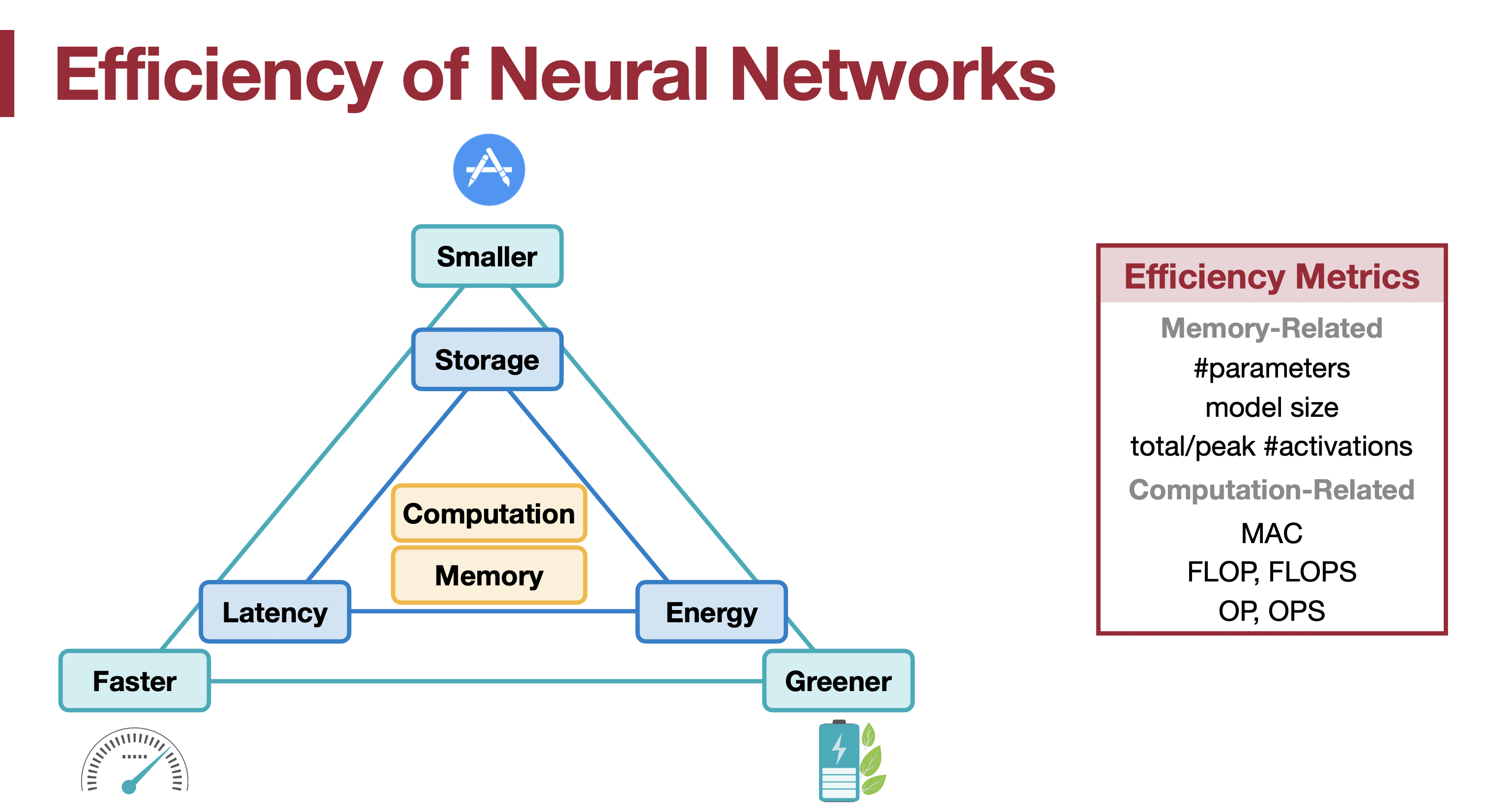
Three pillars of neural network efficiency (Source: MIT 6.5940 Lecture 2)
Why Efficiency Matters
The Deployment Reality Check
Imagine you’ve trained a state-of-the-art image classification model with 99% accuracy. Sounds perfect, right? But then:
Deployment Challenges:
- Your model requires 10GB of memory (mobile phones have 4-8GB total)
- Inference takes 5 seconds per image (users expect <100ms)
- Running it costs $1000/day in cloud compute (budget is $100/day)
- Battery drains in 30 minutes on mobile devices
This is why efficiency matters: a model that can’t be deployed is a model that can’t create value.
Critical Application Areas
Mobile Applications:
- On-device speech recognition (Siri, Google Assistant)
- Real-time camera filters (Instagram, Snapchat)
- Offline translation
Edge Computing:
- Autonomous vehicles (must process 30 frames/second)
- IoT sensors (run on batteries for months)
- Medical devices (limited power, critical latency)
Cloud Services:
- Cost optimization at scale (millions of requests/day)
- Meeting service-level agreements (SLAs)
- Environmental sustainability (reducing carbon footprint)
Latency: The Speed of Response
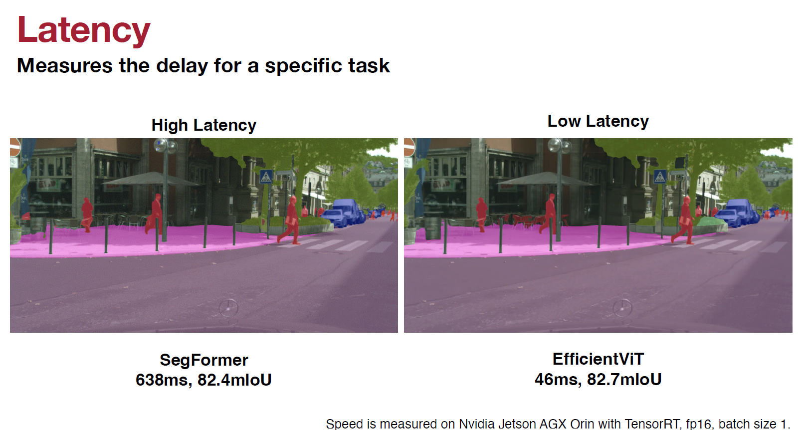
Latency measures delay for specific task completion (Source: MIT 6.5940 Lecture 2)
What is Latency? Latency is the time delay between receiving an input and producing an output. Think of it as the “reaction time” of your neural network.
Analogy: When you ask a friend a question, latency is the time from when you finish asking until they start answering. A quick friend has low latency; a slow friend has high latency.
Components of Latency:
\[\text{Total Latency} = T_{\text{data}} + T_{\text{preprocess}} + T_{\text{inference}} + T_{\text{postprocess}}\]- Data Loading: Reading input from disk or network
- Preprocessing: Resizing, normalization, data augmentation
- Model Inference: Actual neural network computation
- Postprocessing: Formatting output, applying thresholds
Latency Requirements by Application:
| Application Type | Max Acceptable Latency | Why |
|---|---|---|
| Autonomous Driving | <100 ms | Safety-critical decisions |
| Voice Assistants | <200 ms | Natural conversation flow |
| Real-time Translation | <500 ms | Acceptable user experience |
| Batch Processing | Seconds to minutes | No real-time requirement |
Concrete Example: Mobile Image Classification
Scenario: Mobile app that identifies objects through camera
Setup:
- Input: 224×224 RGB image (150 KB)
- Network: ResNet-50 (pre-trained CNN)
- Device: iPhone 12
Latency Breakdown:
1
2
3
4
5
6
Image capture:        10 ms
Preprocessing:        15 ms (resize, normalize)
Model inference:      45 ms (forward pass)
Postprocessing:        5 ms (apply softmax, get top-5)
─────────────────────────
Total latency:        75 ms
Real-Time Requirement Analysis:
- Target: 10 images/second → need <100 ms per image
- Current: 75 ms per image → Meets requirement
- Can handle up to: 1000/75 = 13.3 images/second
What Affects Latency?
Hardware Factors:
- GPU vs CPU: GPU inference typically 5-10× faster
- Memory Bandwidth: Faster RAM reduces data movement time
- Processor Speed: Higher clock rates reduce computation time
Software Factors:
- Batch Size: Processing single samples has overhead
- Optimization Level: Compiler optimizations (TensorRT, ONNX)
- Quantization: INT8 operations faster than FP32
Throughput: Volume Processing Capacity
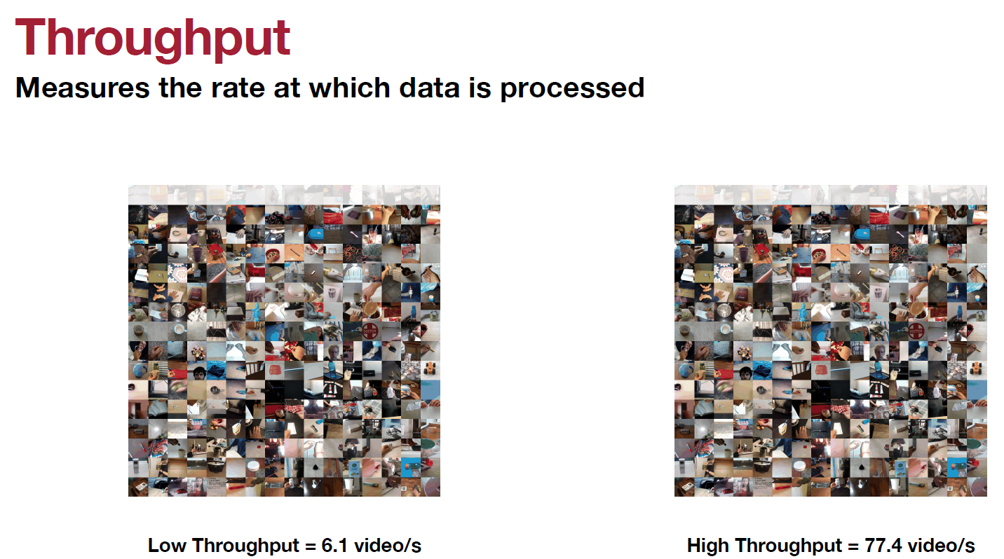
Throughput measures processing rate: 6.1 vs 77.4 videos/sec (Source: MIT 6.5940 Lecture 2)
What is Throughput? Throughput measures how many inputs a system can process in a given time period. It’s about volume, not individual speed.
Analogy: Imagine a restaurant:
- Latency = Time to prepare one order
- Throughput = Total meals served per hour
A restaurant might take 30 minutes per order (high latency) but serve 100 meals/hour by working on multiple orders simultaneously (high throughput).
Throughput Formula:
\[\text{Throughput} = \frac{\text{Batch Size}}{\text{Time per Batch}}\]Measurement Units:
- Samples/second: General metric
- Images/second (IPS): Computer vision
- Tokens/second: Natural language processing
- Queries/second (QPS): API services
Concrete Example: Batch Image Processing
Scenario: Batch image processing for content moderation
Setup:
- Batch size: 100 images
- Processing time: 200 ms per batch
- Hardware: NVIDIA A100 GPU
Calculation:
\[\text{Throughput} = \frac{100 \text{ images}}{0.2 \text{ seconds}} = 500 \text{ images/second}\]Scaling Analysis:
1
2
3
4
Single image (batch=1):    50 ms → 20 images/sec
Small batch (batch=32):   200 ms → 160 images/sec
Large batch (batch=100):  500 ms → 200 images/sec
Optimal batch (batch=256): 1000 ms → 256 images/sec
Cost Impact:
1
2
3
4
5
6
7
8
9
Scenario: Process 1 million images/day

Low throughput (100 images/sec):
  Time: 2.78 hours
  Cost: $50/day

High throughput (1000 images/sec):
  Time: 16.7 minutes
  Cost: $5/day (90% savings!)
Latency vs. Throughput: The Fundamental Tradeoff
Key Differences:
| Aspect | Latency | Throughput |
|---|---|---|
| What it measures | Time per single input | Inputs processed per time unit |
| Units | Milliseconds (ms) | Samples/second |
| Focus | Individual response time | Overall volume |
| Optimization goal | Minimize delay | Maximize capacity |
| Best for | Real-time applications | Batch processing |
The Fundamental Tradeoff:
You can’t optimize both simultaneously—there’s an inherent tension:
Low Latency Strategy:
- Process each input immediately (batch size = 1)
- Minimal waiting time per sample
- Great for real-time, poor for volume
High Throughput Strategy:
- Wait to collect a batch (batch size = 128+)
- Process many inputs together
- Great for volume, poor for individual response time
The Role of Batch Size:
Batch size is the primary control knob for this tradeoff:
| Batch Size | Per-Sample Latency | Throughput |
|---|---|---|
| 1 | 50 ms | 20/sec |
| 8 | 60 ms | 133/sec |
| 32 | 80 ms | 400/sec |
| 128 | 150 ms | 853/sec |
| 512 | 400 ms | 1280/sec |
Pattern: As batch size increases, individual latency worsens, but total throughput improves dramatically.
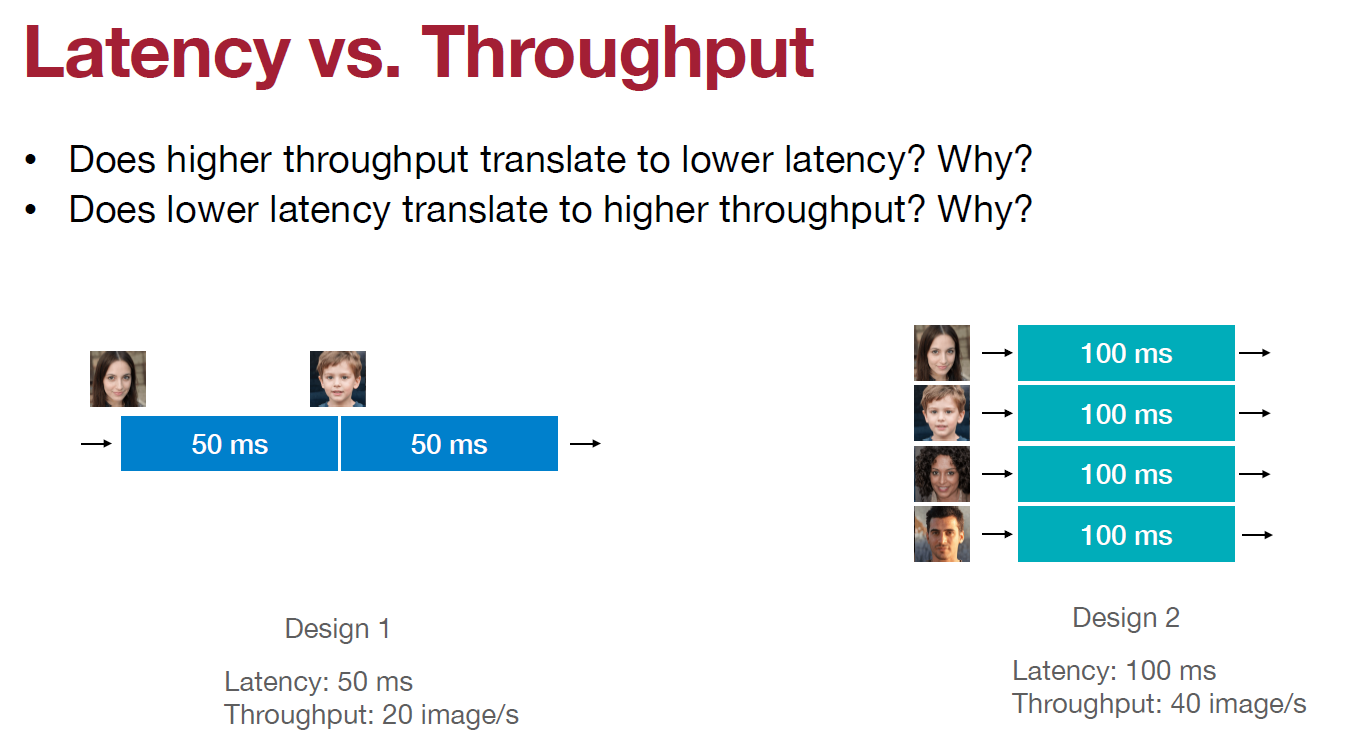
Understanding the fundamental tradeoff between latency and throughput (Source: MIT 6.5940 Lecture 2)
Real-World Application Strategies
Scenario 1: Real-Time Video Processing (Prioritize Latency)
Requirement: Classify video frames for augmented reality
Constraints:
- Must process 30 frames/second
- Each frame needs result <33ms
- User perceives lag above 50ms
Solution:
1
2
3
4
Batch size: 1
Latency: 25 ms per frame
Throughput: 40 frames/sec
Result: Smooth real-time experience ✓
Scenario 2: Bulk Image Classification (Prioritize Throughput)
Requirement: Classify 10 million product images for e-commerce catalog
Constraints:
- Must complete within 24 hours
- No real-time requirement
- Minimize cloud costs
Solution:
1
2
3
4
Batch size: 256
Latency: 200 ms per image
Throughput: 1280 images/sec
Result: Completes in 2.2 hours (saves 22 hours of compute) ✓
Decision Guidelines:
Choose Low Latency When:
- Users are waiting for results
- Real-time decision making required
- Interactive applications
- Safety-critical systems
Choose High Throughput When:
- Batch processing large datasets
- No immediate user interaction
- Cost optimization is priority
- Can tolerate individual delays
Key Takeaways
Performance Metrics Matter: Latency and throughput are the primary performance metrics. They measure different aspects of speed and have different optimization strategies.
The Tradeoff is Fundamental: You cannot optimize for both low latency and high throughput simultaneously. Batch size is the key control parameter.
Application-Driven: There’s no universally “better” metric—it depends entirely on your use case. A self-driving car needs low latency; a photo indexing service needs high throughput.
Beyond Accuracy: Model accuracy alone is insufficient. A 99% accurate model that takes 5 seconds per inference is unusable for real-time applications.
What’s Next?
In Part 2, we’ll explore memory-related efficiency metrics: model parameters, model size, and activation memory—critical for deployment on resource-constrained devices.
Series Navigation:
- Part 1: Performance Metrics (Current)
- Part 2: Memory Metrics
- Part 3: Computation Metrics
References: